Communication and Bargaining Breakdown: An Empirical Analysis

NBER WORKING PAPER SERIES

COMMUNICATION AND BARGAINING BREAKDOWN:

AN EMPIRICAL ANALYSIS

Matthew Backus

Thomas Blake

Jett Pettus

Steven Tadelis

Working Paper 27984

http://www.nber.org/papers/w27984

NATIONAL BUREAU OF ECONOMIC RESEARCH

1050 Massachusetts Avenue

Cambridge, MA 02138

October 2020

We are grateful to numerous seminar and conference participants, as well as to Charles

Angelucci, Anne Bartel, Wouter Dessein, Liran Einav, Sarah Moshary, Michaela Pagel, Andrea

Prat, and especially Jonah Rockoff for thoughtful comments, as well as many eBay employees for

their input and support, and finally Brenden Eum and Alphonse Simon for excellent research

assistance; all remaining errors are our own. Part of this research was supported by NSF Grant

SES-1629060. Matt Backus has in the past been a paid consulting researcher for eBay Inc. The

views expressed herein are those of the authors and do not necessarily reflect the views of their

employers, eBay, or the National Bureau of Economic Research.

NBER working papers are circulated for discussion and comment purposes. They have not been

peer-reviewed or been subject to the review by the NBER Board of Directors that accompanies

official NBER publications.

Short sections of text, not to exceed two paragraphs, may be quoted without explicit permission

provided that full credit, including © notice, is given to the source.

Communication and Bargaining Breakdown: An Empirical Analysis

Matthew Backus, Thomas Blake, Jett Pettus, and Steven Tadelis

NBER Working Paper No. 27984

October 2020

JEL No. C78,D82,D83,M21

ABSTRACT

Bargaining breakdown—whether as delay, conflict, or missing trade—plagues bargaining in

environments with incomplete information. Can a bargaining environment that facilitates or

restricts communication alleviate these costs? We exploit a unique opportunity to study this

question using real market transactions: eBay Germany’s Best Offer platform. On May 23, 2016,

the platform introduced unstructured communication allowing buyers and sellers on the desktop

version of the site, but not the mobile app, to accompany price offers with a message. Using this

natural experiment, our difference-in-differences approach documents a 14% decrease in the the

rate of breakdown among compliers. Though adoption is immediate, the effect is not. We show,

using text analysis, that the dynamics are consistent with repeat players learning how to use

communication in bargaining, and that the messaging strategies of experienced sellers are

correlated with successful bargaining.

Matthew Backus

Graduate School of Business

Columbia University

3022 Broadway, Uris Hall 619

New York, NY 10027

and NBER

[email protected]

Thomas Blake

eBay Research Labs

2065 Hamilton Ave

San Jose, CA 94125

[email protected]

Jett Pettus

Columbia University

[email protected]

Steven Tadelis

Haas School of Business

University of California, Berkeley

545 Student Services Building

Berkeley, CA 94720

and NBER

[email protected]

1 Introduction

Bargaining is the mechanism of choice for many of our most important transactions:

peace negotiations, federal budgets and the formation of governing coalitions, allocation

of refugees, the sale of a business, the purchase of a car, child care duties, and the

number of bedtime stories, to name a few. Yet at least since Myerson and Satterthwaite

(1983), economists have understood the potential for failure in bargaining. When

parties to a negotiation do not know each other’s reservation values, each has an

incentive to overstate the strength of their position to get a better deal, sometimes

resulting in costly delays, and other times in a complete loss of socially beneﬁcial trades.

In this spirit, Crawford (1982) posits that “the potential welfare gains from improving

the eﬃciency of bargaining outcomes are enormous, perhaps even greater than those

that would result from a better understanding of the eﬀects of macroeconomic policy.”

We consider an open question in this domain: does communication improve the

eﬃciency of bargaining outcomes, or is it all “cheap talk?” Charness (2012) writes:

For many, the word bargaining conjures an image of people sitting around

a table talking. Yet communication is one of the least understood facets

of bargaining. Most economic models of bargaining assign no role for

communication beyond conveying oﬀers or their acceptability. But clearly,

communication does a lot more than that.

He continues, presciently, “this area should be of great importance in the coming

years, particularly given the strong trend to virtual interaction in bargaining.” Here,

we oﬀer evidence on this question using data from such a virtual bargaining platform:

eBay’s Best Oﬀer bargaining marketplace. We present two main ﬁndings: ﬁrst, we

document a statistically and economically signiﬁcant positive relationship between the

availability of free-form text communication and bargaining success. Second, applying

text analysis techniques to users’ messages, we document a convergent pattern which,

we argue, represents repeat players learning how to communicate in the bargaining

protocol. We show that this pattern is related to experience, and that the strategies

adopted by experienced bargainers are correlated with successful negotiation. This is

consistent with prior ﬁndings in experimental work demonstrating that beyond the

ability to communicate, the content of communication matters as well for bargaining

outcomes. Our work is, to the best of our knowledge, the ﬁrst study of the role of

communication in bargaining using data from real-world bargaining interactions.

Our ﬁndings relate to a broader debate concerning the restriction of communication

in bargaining which, in practice, is quite common. A high stakes example from

international relations is “shuttle diplomacy,” which played a high-proﬁle role in many

negotiation episodes in the twentieth century. Theoretical models of such mediation,

itself a medium of communication, focus on the informational role of these restrictions,

as against the theoretical limitations of baseline of unveriﬁable cheap talk (Fey and

Ramsay, 2010; H¨orner et al., 2015). Yet these theoretical limitations oﬀer limited

perspective on real-world bargaining, which is rife with cheap talk (very little of which,

in our setting, resembles meaningful exchange of information).

This is particularly salient for marketplaces, where bargaining is increasingly

commonplace. eBay’s Best Oﬀer bargaining platform, which allows sellers to receive

and respond to oﬀers from potential buyers, accounts for approximately 10% of eBay’s

trade volume, which was

84 billion globally in 2016.

On the Chinese platform

TaoBao, which hosted trade volumes of

115 billion in 2016, bargaining is the standard

for all transactions.

And in, in 2014, Amazon.com introduced their own bargaining

mechanism for the Amazon Marketplaces platform called “Make an Oﬀer.” All of

these platforms face the question of how and whether to regulate communication.

Our setting is the Best Oﬀer bargaining platform on eBay.de, the German counter-

part of eBay.com.

Sellers who create a listing on the website may enable Best Oﬀer,

a free feature that allows buyers to make oﬀers below the listing price. An oﬀer may

be countered, and the counter-oﬀer countered, etc., yielding a protocol very similar

to sequential, alternating-oﬀers bargaining (Rubinstein, 1982). Originally, eBay.de

did not allow communication, and only numerical oﬀers were relayed between the

parties.

However, in a policy change that took eﬀect May 23, 2016, oﬀers could

be accompanied by a 250-character message when made from the eBay.de website.

Importantly, the change did not aﬀect buyers who made oﬀers using their mobile

devices. The sudden nature of the change and its incomplete coverage aﬀords us a

natural experiment to study the role of communication in bargaining.

See Backus et al. (2020) and eBay’s 2016 10k SEC ﬁling.

On TaoBao, communication is encouraged between buyers and sellers on an instant messenger

service. This has been cited as a factor in their success over the Chinese equivalent of eBay

(Oberholzer-Gee and Wulf, 2009).

This platform is also used in Gizatulina and Gorelkina (2017), who conduct a ﬁeld experiment

selling gift cards on the platform to study surplus division.

We believe this has to do with the origins of eBay.de, which was originally developed by Rocket

Internet SE in 1999 and then sold to eBay.com. Thanks to Ariel Stern for pointing this out.

We ﬁnd that, while the typical bargaining session in our sample was successful forty-

four percent of the time, bargainers who used messages were eight percentage points

more likely to transact than they would have been in the absence of communication.

This corresponds to a fourteen percent reduction in the rate of bargaining breakdown.

We do not observe bargainers’ private values, so “breakdown” is not the same as

ineﬃciency (e.g., if a seller values the product more than the buyer, then breakdown

is an eﬃcient outcome). Therefore our computation is conservative in the sense that

the denominator is too large—the decrease in the rate of ineﬃcient breakdown is

likely to be much larger. Additionally, examining week-speciﬁc eﬀects, we ﬁnd that

the eﬀect of communication grows gradually over the four weeks after introduction.

One mechanism that may drive this pattern is that it takes time for players to learn

how to best make use of the new feature after the change.

To explore this mechanism, we implement a descriptive analysis of the content of

the communications. Most notably, we oﬀer evidence that over the weeks following

the introduction of communication, sellers’ communication strategies evolve as they

learn to use the communication feature in bargaining. In contrast, the content of

buyers’ communications is largely random, which is consistent with our intuition, and

their behavior on eBay, that they are occasional, short-run players. We show that not

only are repeat sellers’ strategies changing over time, but that they are convergent,

supporting the hypothesis that they are learning. Consistent with this, we show that

messages most similar to the endpoint of that convergence are more likely to succeed,

with a magnitude that is remarkably close to our estimates of the treatment eﬀect on

the treated from the introduction of messaging. We also, in an Appendix, borrow tools

from text analysis to learn about what sellers are converging to; though this analysis is

entirely descriptive, the ﬁndings are consistent with behavioral and experimental work

which shows that cost-based rationales are eﬀective, and overly eﬀusive communication

strategies can be counterproductive.

Turning to prior work, our paper is the ﬁrst, to the best of our knowledge, to study

the role of communication on bargaining using real-world bargaining interactions.

There is, however, substantial prior theoretical and experimental work. Surveying

theoretical contributions, Crawford (1990) distinguishes between tacit and explicit

models of bargaining, where tacit models leave no role for communication. All of

noncooperative bargaining theory is tacit; it abstracts away from talk to focus on

actions: oﬀers, counteroﬀers, delay, agreement, and exit. For practitioners, however,

haggling and negotiation are understood as communication, which may explain the

minor role of economic theory in negotiation coursework among students of law and

business. More recent work studies explicit bargaining, in which communication

is modeled as cheap talk.

There is signiﬁcant disagreement on the eﬃciency of

allowing cheap talk: theoretical work predicts that, among rational actors, it is at

best irrelevant, and possibly detrimental to bargaining eﬃciency.

In the latter case

restricting communication is a form of pre-commitment, which may improve outcomes.

In contrast, experimental work has found potential for communication to improve

outcomes in bargaining among other games.

Indeed, bargaining experiments that

manipulate the availability of communication (Radner and Schotter, 1989; Valley et

al., 2002) oﬀer evidence that communication may permit bargaining eﬃciency that

exceeds the theoretical upper bounds outlined by Myerson and Satterthwaite (1983).

However, these results have not been validated in the ﬁeld, and subsequent extensions

are not uniformly positive: Ert et al. (2014) construct an experimental scenario with

misalignment of incentives, similar to bargaining over lemons, where communication

elicits skepticism and increases breakdown; Bolton et al. (2003) and McGinn et al.

(2012) highlight drawbacks of communication in bargaining games with more than

two players, and Lee and Ames (2017) and Jeong et al. (2019) show how the content

of the messages can facilitate or inhibit negotiations.

Communication is of interest for antitrust economics, where colluding parties have

to bargain over the division of surplus. Cooper and K¨uhn (2014) experimentally study

the role of communication in repeated Prisoners’ Dilemma games; Awaya and Krishna

(2015) show how cheap-talk communication can overcome the problem of secret price

cuts in collusive arrangements, and Harrington and Ye (2019) show how cheap-talk

This literature typically appends a cheap-talk “pre-game” to an existing bargaining model. See,

e.g., Farrell and Gibbons (1989), Cabral and S´akovics (1995), for early examples, and Menzio (2007)

for a formalization of partially directed search in models of cheap-talk wage-posting.

See Goltsman et al. (2009) for a treatment and review of communication and bargaining in the

cheap-talk setting described by Crawford and Sobel (1982), and, in the legal literature, Brown and

Ayres (1994) and Ayres and Nalebuﬀ (1997).

In experiments mirroring Crawford and Sobel (1982), Cai and Wang (2006) ﬁnd that subjects

consistently reveal “too much” information to be rationalized by equilibrium behavior. This is

consistent with lie aversion (Gneezy, 2005; Gibson et al., 2013) and guilt aversion (Charness and

Dufwenberg, 2006, 2011), as well as communication fostering other-regarding preferences (Coﬀman

and Niehaus, 2020). Crawford et al. (2013) argue that it is consistent with level-K thinking, even in

the absence of preferences for truthfulness, as L0 types anchor on the truth. In games with multiple

equilibria, communication helps coordination on better outcomes (Cooper et al., 1992; Blume and

Ortmann, 2007; Ellingsen and

Ostling, 2010). McGinn et al. (2003) oﬀer evidence for this mechanism

by showing that communication elicits dyadic strategies by bargainers.

communication among sellers in an upstream market can facilitate collusion when

the downstream market is characterized by negotiations, as in many intermediate

goods markets. Clark and Houde (2014) oﬀer an empirical example of the role of

communication in collusion, studying the collapse of a cartel resulting from antitrust

enforcement equipped with a wire tap in Quebec. Moreover, in a setting that features

on-path bargaining breakdown but not communication, Loertscher and Marx (2020)

show how mechanism design can be used to understand bargaining and countervailing

power in antitrust.

Finally, our work contributes to the literature on learning in strategic settings.

Empirical work in this area is particularly scarce because there are few opportunities to

observe the introduction of a novel mechanism in a continuously operating marketplace.

In this respect, our work is related to Doraszelski et al. (2017), who document bidding

behavior in a newly opened electricity auction market. Our exercise builds on the

recent introduction of text analysis and natural language processing; see Gentzkow

et al. (2019a) for a survey. For the same reason that we need new tools to study

text—that messages live in a high-dimensional space—we conjecture that it is a natural

environment to study learning and experience.

Section 2 describes the eBay.de platform, and Section 3 describes the dataset and

explain the motivation for the sample design. Section 4 oﬀers a discussion of identiﬁ-

cation and our main causal estimates of the eﬀect of communication on bargaining

breakdown. Section 5 presents a descriptive analysis of the text communication itself

in order to match the patterns we ﬁnd, and Section 6 shows that our text analysis

ﬁndings are consistent with message-level regressions predicting successful bargaining.

Finally, Section 7 concludes with a brief discussion of the implications for platforms

and future directions for empirical work on communication and bargaining.

Though no prior work isolates the interaction of communication and experience in bargaining,

there is evidence of the importance of experience in bargaining: see, e.g. Card and Dahl (2012), who

documented the role of expertise in bargaining agents in arbitration, and Backus et al. (2020), who

found eﬀects of experience on bargaining outcomes on eBay.com.

Figure 1: Example of a Best Oﬀer Listing

Notes: This is an example View Item page for a Best-Oﬀer enabled listing. A buyer may purchase at the asking price

of $55 by clicking the Buy-It-Now button, or they may engage in bargaining by clicking the Make Oﬀer button.

2 Our Empirical Setting: Bargaining on eBay.de

2.1 Best Oﬀer Bargaining

eBay’s online platform matches buyers to sellers who sell products ranging from art

and collectibles to mobile phones, with over

95 billion dollars in gross merchandise

volume worldwide in 2018. The platform operates in many markets throughout the

world, the largest by revenue are the US (eBay.com) and Germany (eBay.de).

Sellers who list an item choose either an auction or ﬁxed-price (“Buy-it-Now”)

format. We focus on a subset of ﬁxed-price listings for which the seller enables the

“Best Oﬀer” bargaining feature as shown in Figure 1. A buyer considering this listing

has two options to purchase the good: they can either purchase at the posted asking

price (here,

55), or they can oﬀer to purchase at a lower price. If the buyer makes an

oﬀer, the seller is notiﬁed and they may then accept, decline, or make a counter-oﬀer. If

the seller makes a counter-oﬀer, the buyer may accept, decline, or make a counter-oﬀer,

and so on, in the spirit of Rubenstein-St¨ahl alternating, sequential-oﬀers bargaining.

Oﬀers by either party expire automatically after 48 hours.

Figure and revenue ranking based on eBay’s 2018 Annual Report.

For a more thorough descriptive characterization of the Best Oﬀer environment, see Backus et al.

(2020). Data from that study, which are collected from the US site eBay.com, are publicly available

at http://www.nber.org/data/bargaining/.

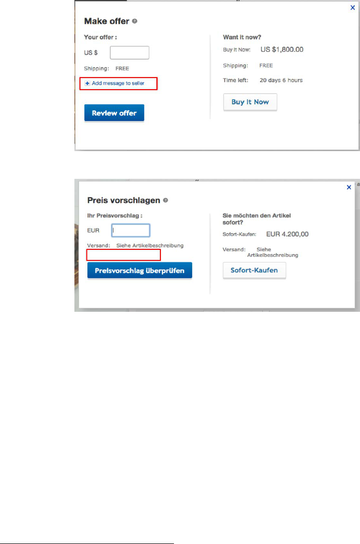
Figure 2: Messages and Best Oﬀer

(a) eBay.com

(b) eBay.de (before May 23, 2016)

Notes: Panel (a) depicts the “Make Oﬀer” panel for eBay.com, the US site, where we have highlighted the “add

message to seller” button. Panel (b) depicts the pre-treatment panel on eBay.de, where there is no option to send a

message.

The Best Oﬀer bargaining mechanisms on eBay.com and eBay.de are mostly

identical except for one peculiarity that was unique to eBay.de up until the policy

change we study: bargainers weren’t allowed to communicate like on eBay.com. Figure

2(a) depicts the “Make Oﬀer” interface through which buyers submit their oﬀer, for

eBay.com. If a buyer clicks the “add message to seller” button, they may include

a free-form text message of up to 250 characters which will accompany their oﬀer.

Figure 2(b) depicts the parallel “Preis Vorschlagen” interface, for eBay.de. The red

rectangle highlights where the missing option to send a message might have been.

The reason for the diﬀerence is unclear, but it may be a historical artifact: eBay.de is the

successor of Alando.de, a clone of eBay.com created by the company Rocket Internet in 1999. 100

days after its creation, it was sold to eBay for

43 million. Thanks to Ariel Stern of HBS for pointing

this out.

2.2 The Policy Change: May 23, 2016

On May 23, 2016, the “add a message to seller” feature was added to eBay.de’s Best

Oﬀer bargaining platform. However, the rollout on that date was partial. The website

eBay.de was updated, but the app for mobile users was not.

The policy change aﬀords the main source of variation that we will exploit in this

paper. Unlike many changes to the eBay platform, the introduction of messaging

on eBay.de was not accompanied by a far-reaching “seller update”, and no other

major changes to the eBay.de experience happened around this change. Moreover,

the availability of an untreated group in the post period (mobile users) aﬀords us a

control group in order to separate changes in behavior from a secular trend.

3 Dataset and Sample Design

We obtained proprietary data from eBay itself to evaluate the eﬀect of messaging

on bargaining breakdown. We study bargaining interactions, which we deﬁne as a

buyer-item pair in which we observe at least one oﬀer. Our main dataset includes all

interactions for which the ﬁrst buyer oﬀer was made during an eight-week window

between April 26, 2016 and June 20, 2016, constructed to be four weeks before and

four weeks after the introduction of messaging on May 23, 2016.

3.1 Summary Statistics

Table 1 presents summary statistics for the main sample across several dimensions:

listings, buyers, sellers, and interactions. This sample includes 3.3 million interactions

involving 2.2 million unique listings, 444 thousand sellers, and 1.6 million buyers. The

listings span all categories of eBay excluding real estate, automobiles, and tickets. As

documented by Backus et al. (2020), Best Oﬀer is more frequently used in categories

with substantial heterogeneity, such as Collectibles. Listings observed in our sample

have on average 1.5 interactions (note that our sample excludes listings with zero

interactions) and the distribution is highly skew: 79 percent have only one; 91 percent

have two or fewer, 96 percent have three or fewer, and there is a right tail with many

more.

55 percent ultimately sell through the Best Oﬀer mechanism.

Both buyers and sellers may be involved in multiple interactions—on average, 2.1

and 7.4, respectively. In both cases there is substantial positive skew, suggesting a

large right-tail of highly-active participants. On the buyer side, this derives from the

fact that most (60%) are only observed in a single interaction, while the top decile

participates in four or more interactions. On the seller side, only 34% of the sample is

observed only once, while the top decile participates in twelve or more interactions.

This diﬀerence motivates our interpretation of buyers as short-run players and sellers

as long-run players. These patterns hold for sales and purchases as well.

At the interaction level, which is the unit of observation for the empirical analysis

that follows, we see that 44% of interactions end in a sale. These facts are consistent

with ﬁndings in prior work using data from the U.S. site eBay.com (Backus et al.,

2019, 2020). The ﬁnal two interaction-level variables of Table 1 are of unique interest

to this paper: interactions may be initiated by buyers using the desktop version of

eBay (54%) or the mobile version (46%), which is important because only desktop

buyers have the opportunity to send messages after the policy change. Finally, 50% of

our sample falls after the policy change on May 23, 2016.

3.2 Additional Controls

In addition to the basic characteristics summarized in Table 1, we have a number of

controls available to predict bargaining breakdown. These include the asking price of

the seller; dummy variables by product category and condition (new, used, refurbished,

or unknown); and dummy variables for the day of the week on which the ﬁrst oﬀer in

an interaction is made (to allow for diﬀerential behavior on weekends and weekdays);

a “holiday” dummy, which encodes all publicly observed holidays in Germany, as

there is a particularly large number of them in May.

We also include controls for the

weather in Frankfurt, Hesse, which we expect to be correlated with weather elsewhere

Partly for this reason, and partly because Best Oﬀer listings tend to take longer to sell than, say,

auctions, we ignore the possibility of competing oﬀers by buyers. This is intuitive, since sellers also

have the option to hold an auction on the eBay platform.

Listings that sold at the Buy-it-Now price are not classiﬁed as an interaction because no

negotiation is involved. These sales do not appear in our dataset.

Publicly observed holidays in our sample include: May 1, Labor day; May 5, Ascension Day;

May 8, Mother’s Day; May 16, Whit Monday, and May 26, Corpus Christi.

Table 1: Summary Statistics

Mean Std. Dev. Skewness Min Max

Listing-Level Data

Asking Price (USD) 100.6 151.5 2.889 1.050 999.9

Number of Interactions 1.490 2.566 82.62 1 1004

1(Sold) 0.563

N 2210575

Seller-Level Data

Number of Interactions 7.426 42.30 47.81 1 7142

Number of Sales 3.279 20.76 44.17 0 3115

N 443644

Buyer-Level Data

Number of Interactions 2.101 3.102 20.24 1 396

Number of Purchases 0.928 1.526 25.26 0 389

N 1567995

Interaction-Level Data

Number of Oﬀers 1.873 1.116 1.535 1 6

1(Ended in Sale) 0.442

1(Buyer on Desktop) 0.537

1(First oﬀer after May 23) 0.501

N 3294362

Notes: This table presents summary statistics for the main dataset of Best Oﬀer interactions taking place within an

eight-week window, four weeks before and four weeks after the policy change on May 23, 2016. Fixing that set of

interactions, we have constructed the summary statistics four ways: where the unit of observation is the listing (i.e.,

the product), the buyer, the seller, or the interaction itself.

in Germany, as weather conditions are both serially correlated and anecdotally cited

as aﬀecting online activity. These include a dummy for precipitation as well as the

deviation of temperature from a linear trend over the sample.

3.3 Adoption on May 23, 2016

As depicted in Figure 3(a), users adopted messages rapidly: within days, the hazard

rate with which bargaining interactions by desktop-only buyers involved messaging

stabilized at approximately six percent. Both panels in Figure 3 distinguish between

the case where the buyer is either exclusively making oﬀers from a desktop computer

or exclusively making oﬀers from a mobile device. We do this because there was

initially no messaging feature for the eBay.de mobile app. Therefore in Panel (a),

which plots the hazard rate at which interactions involve any message (both seller and

buyer messages), the hazard rate for the case where the buyer is on the mobile app is

much lower. These are exclusively messages sent by sellers, to mobile-only buyers who

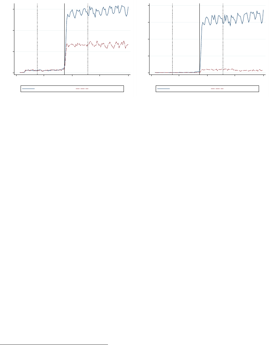
Figure 3: Launch of Messaging Feature

0 .02 .04 .06

Fraction with Any Message

01apr2016 01may2016 01jun2016 01jul2016 01aug2016

Time

Buyer is Desktop Only Buyer is Mobile Only

(a) Any Message

0 .01 .02 .03 .04

Fraction with Buyer Message

01apr2016 01may2016 01jun2016 01jul2016 01aug2016

Time

Buyer is Desktop Only Buyer is Mobile Only

(b) Buyer Message

Notes: Panel (a) depicts the fraction of interactions, by ﬁrst oﬀer date, in which a message was included by the seller.

Panel (b) restricts attention to cases where the message was sent by a buyer. Both panels split the sample by whether

the buyer was active on the desktop or mobile version of the platform. The solid vertical line represents the policy

change. Dashed vertical lines depict the bounds of the eight-week window, centered at launch, of our main sample.

cannot read them. In Panel (b), we plot the hazard rate of buyer messages, which

conﬁrms that mobile-only buyers are not sending messages after the change.

4 The Eﬀect of Introducing Communication on

the Likelihood of Bargaining Breakdown

4.1 Empirical Design and Identiﬁcation

4.1.1 OLS and Endogeneity

Our identiﬁcation strategy is meant to circumvent the most salient problem, that the

choice to include a message is endogenous. In particular, we expect a negative bias:

that bargainers send messages for goods of a type where bargaining is least likely to

succeed, or in order to motivate a particularly aggressive oﬀer.

We illustrate this by estimating a linear probability model, the details of which

can be found in Appendix Section A. The unconditional correlation between the

About 0.1% of oﬀers per day included messages prior to the feature launch, and similarly there

are cases where mobile-only buyers appear to send messages. In the former case, these are seller-side

only, and rarely in German, so we believe that they are anomalies related to sellers registered on

multiple sites. In the latter, we believe that these are simple database errors.

presence of a message and bargaining success is negative, but once we condition

on the log of the asking price it is small and positive. This reﬂects the fact that

bargaining interactions with messages tend to involve goods that are more expensive

than bargaining interactions that do not, and that bargaining success is less likely for

more expensive products, as documented by Backus et al. (2020) for eBay.com.

We expect this problem to be at least as important for unobservable characteristics

than the asking price, and therefore rely on the policy change for a natural experiment

and a more credible estimate of the eﬀect of communication on bargaining breakdown.

4.1.2 Identiﬁcation

The variation generated by the May 23, 2016 policy change allows us to identify the

eﬀect of communication in two ways. The ﬁrst is a simple pre-post design studying

the change in the mean success rate of bargaining interactions before and after the

policy change among desktop users. Our dependent variable is

(success), a dummy

for whether the bargaining interaction ends in a sale. Let

denote a set of controls,

(alternatively, “post”) a dummy equal to one if the ﬁrst oﬀer in an interaction is in

the post period, and

(alternatively, “desktop”) a dummy equal to one if the buyer

makes oﬀers from the desktop version of eBay.de. Then, the pre-post estimate of the

eﬀect of communication on bargaining success is given by:

= E[1(success)|X, P = 1, D = 1] − E[1(success)|X, P = 0, D = 1]. (1)

We can then use the untreated set of buyers who made oﬀers on the mobile

platform—where messaging was unavailable both before and after May 23, 2016—to

control for common trends and alleviate concerns of endogeneity. This suggests a

diﬀerences-in-diﬀerences design:

=(E[1(success)|X, P = 1, D = 1] − E[1(success)|X, P = 0, D = 1]) (2)

− (E[1(success)|X, P = 1, D = 0] − E[1(success)|X, P = 0, D = 0]).

Both of the above strategies identify an eﬀect that should be interpreted as an

intent to treat (ITT) estimate, i.e., an estimate of the eﬀect of the availability of

communication, rather than the eﬀect of actually choosing to communicate. In order

Table 2: Complier Characteristics

P(x=1) P(x = 1 | complier)

P(x=1|complier)

P(x=1)

Ask Price in ($0,$50) 0.52 0.41 0.78

Ask Price in [$50,$150) 0.27 0.29 1.08

Ask Price in [$150,$250) 0.09 0.11 1.30

Ask Price ≥ $250 0.12 0.19 1.54

Friday, Saturday, or Sunday 0.42 0.42 1.00

Precipitation 0.46 0.67 1.46

Holiday 0.10 0.03 0.32

Post 0.50 1.00 2.00

Desktop 0.54 1.00 1.86

Notes: This table summarizes complier characteristics, i.e. the characteristics of interactions in the treatment group

that “comply” and involve a message between bargainers. Each row represents a dummy variable which is taken to

be x in the column formulas above.

to identify the treatment eﬀect on the treated (TOT), we need to clarify who the

compliers, i.e., those we actually consider to be treated, are.

4.1.3 ITT and TOT: Who are Compliers?

We say that a bargaining interaction is in the ITT group if the ﬁrst oﬀer occurs after

May 23, 2016 and if the buyer uses the desktop version of eBay.de. Not every such

interaction involves a message. By deﬁnition, compliers are interactions in our ITT

group in which a message is sent by either party. Some messages were sent outside of

this group, e.g., when a seller sends a message to a buyer who is using the mobile app.

We exclude these for two reasons: ﬁrst, because the buyer was mechanically unable

to read the message, and second, because it turns out that using this less-restrictive

deﬁnition will cause us to overstate the magnitude of the TOT estimate.

Table 2 summarizes the characteristics of the compliers. Of particular note is the

fact that bargainers are more likely to send messages when the asking price is higher,

consistent with the intuition that communication is costly. The higher likelihood of

precipitation and lower likelihood of a holiday is due mostly to early-May holidays and

late-May rains, and we note that weekend users are no more likely to send messages.

Results are available on demand from the authors, however the intuition is simple: including

messages in the pre-period or mobile set but not in the intent-to-treat group will inﬂate the coeﬃcients

(Post) and

(Desktop), respectively, and thereby depress the coeﬃcient on

(Post)

·1

(Desktop).

Since the ﬁrst-stage coeﬃcient (which is in the denominator) is smaller, the IV eﬀect will be inﬂated.

Including all non-ITT messages will approximately double the estimate.

We group Friday, Saturday, and Sunday based on the OLS coeﬃcients reported in Table A-1,

where weekends appear to be discretely diﬀerent from weekdays.

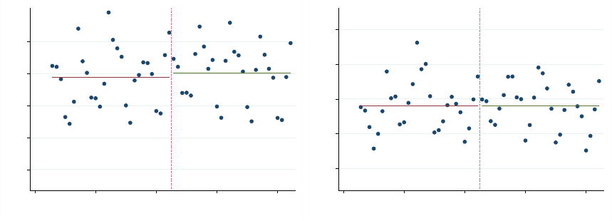
Figure 4: Predicted Success Rates

.44 .45 .46 .47 .48

Predicted Probability

22apr2016 06may2016 20may2016 03jun2016 17jun2016

Day

(a) Desktop

.39 .4 .41 .42 .43

Predicted Probability

22apr2016 06may2016 20may2016 03jun2016 17jun2016

Day

(b) Mobile

Notes: Panel (a) depicts predicted success rates using a large set of controls (ln(ask price); category by condition

ﬁxed eﬀects; day of week, precipitation, and holiday dummies and the temperature) for desktop users only. Panel (b)

replicates this for the mobile users. The vertical axes on both plots are scaled identically subject to a location shift.

It is natural to wonder whether despite our controls, unobservable characteristics

of the listings are generating compositional diﬀerences in the periods before and after

the change. Therefore, in Figure 4 we document the predicted success rate conditional

on those controls for all interactions for both samples—mobile and desktop—where

the ﬁrst-stage regression excludes the dummy for treatment as well as the time trend.

We see a small change in the predicted likelihood of success for desktop users and none

for mobile users, so we anticipate slightly smaller eﬀects when we include controls.

4.2 Empirical Results

4.2.1 Regression Analysis

In what follows, we ﬁrst generate precise estimates

and

, and second, we identify

a treatment eﬀect on the treated because, recall from Figure 3, only a small fraction

of interactions in the post period involve a message. To accomplish the former, we

reformulate (1) and (2) in terms of a linear probability model and estimate them using

OLS (in all of what follows we omit observation indices):

1(success) = β

+ Xβ

+ P β

+ ε, (3)

and

1(success) = β

+ Xβ

+ P β

+ Dβ

+ P Dβ

+ ε. (4)

Next we consider the treatment eﬀect on the treated. We estimate this by reformulating

(4) as an instrumental variables regression:

1(success) = β

+ Xβ

+ P β

+ Dβ

+ 1(complier)β

+ ε, (5)

where

P · D

is an instrument for

(complier), and

(complier) is a dummy for

interactions in the ITT group that include a message. Importantly, this does not

employ any variation that is not already used in the diﬀerences-in-diﬀerences estimator.

Instead, it just rescales the estimate to the end of interpreting its economic meaning.

As with all estimates of the treatment eﬀect on the treated, it should be interpreted

with caution, as bargainers’ decision of whether to send a message is endogenous.

Results for each of these three estimators, both with and without the controls

discussed in Section 2, are presented in Table 3. We see a large eﬀect of the policy

change on success for desktop users, 0.46 percentage points in model (1), which is

attenuated by the inclusion of controls to a statistically insigniﬁcant eﬀect of 0.23

percentage points in model (2). As we show in the next section, the control that

attenuates the result is the time trend. In the post period, there is a substantial

positive drift, which stabilizes after a few weeks. Is this a delayed treatment eﬀect, or

a secular trend on the platform? To distinguish between these hypotheses, we need a

suitable control group; here, interactions involving buyers who use the mobile app.

Critically, as we see in models (3) and (4), our estimates of

for the placebo

sample of mobile users are very close to zero. Therefore, diﬀerences in diﬀerences

estimates in models (5) and (6), where the relevant estimate is the term on the

interaction eﬀect, are of the same order as those in (1): we estimate eﬀects of 0.40

and 0.42, respectively. In particular for speciﬁcation (6), with the rich set of controls,

the mobile group is distinguishing common time trend from the ITT estimate.

Finally, models (7) and (8) report the IV estimates which are rescaled to obtain the

TOT estimate. As only a small fraction of users, approximately six percent, actually

send messages in the post period, this means that the roughly half-percent eﬀect on

conversion for the Best Oﬀer environment at large translates to a substantially larger

and economically important eﬀect on the treated. To be precise, versus a baseline

probability of success near 44% for the full sample (from Table 1), interactions that

involve messages in the treated group are 7.44 (or 7.73, with controls) percentage

points more likely to succeed. The inclusion of these controls (time trend; ln(ask price);

category by condition ﬁxed eﬀects; day of week, precipitation, and holiday dummies

and the temperature) allows us to rule out the most salient alternative hypotheses

by which the eﬀect is driven by compositional changes spurred by the introduction

of communication, e.g. if messaging prompts buyers to bargain over cheaper goods

which also have lower rates of breakdown. This leaves is with our main result: a 14%

decrease in the rate of bargaining breakdown among the compliers.

Finally, a note on size and power: we are looking at extremely small eﬀects, on

the order of half a percentage point. They are small because take-up of the messaging

feature among the ITT group, i.e., the compliance rate, is low, at approximately six

percent. While we have a lot of data in our main sample—3.41 million bargaining

interactions—this turns out to be close to what we need. Simple power calculations for

the detection of an eﬀect of 0

005 with a baseline success rate of 0

442 (borrowed from

Table 1) with a conﬁdence of

= 0

05 and a power of ﬁfty percent implies that we

need a dataset of 2.72 million experimentally generated observations equally divided

between treated and not. Therefore there are limitations on how far we can push the

data to understand heterogeneity in the eﬀects of communication.

While the low compliance rate is, in that sense, an empirical challenge, there is

also a sense in which it is an advantage of our environment. If the greater fraction

of buyers sent messages—and those messages were important for bargaining—then

their communication might have an equilibrium eﬀect on the quantity, composition,

or listing style of goods on the platform. In the language of Angrist et al. (1996),

these are concerns about the stable unit treatment value assumption (SUTVA)—i.e.,

that treatment of some observations has spillover eﬀects on the eﬀectiveness of the

treatment for others. The fact that the compliance rate is very low reassures us that

they are not economically signiﬁcant, and that we can identify a partial equilibrium

eﬀect, i.e. conditional on the broader state of eBay.de in the Summer of 2016.

4.2.2 Graphical Intuition

In order to oﬀer some intuition for the results in Table 3, Figure 5 presents the data

aggregated to the daily level, both with and without residualization on a large set of

controls.

In both cases we see an apparent jump in the success rate of approximately

Note that while we will include it in the regression analysis that follows, we have excluded a

time trend from the set of controls here. Coeﬃcients from the OLS regression that generates these

residuals are reported in model (6) of Table A-1 in the appendix, where we present OLS results as a

straw man alternative to our empirical design.

Table 3: Eﬀect of Messaging on Success Rate

Desktop Mobile Diﬀerences IV

(1) (2) (3) (4) (5) (6) (7) (8)

1(Post) 0.0046

∗

0.0023 0.0006 0.0031 0.0006 0.0005 0.0006 0.0009

(0.0013) (0.0019) (0.0013) (0.0019) (0.0013) (0.0015) (0.0013) (0.0015)

1(Desktop) 0.0599

∗

0.0482

∗

0.0599

∗

0.0482

∗

(0.0013) (0.0011) (0.0013) (0.0011)

1(Post) · 1(Desktop) 0.0040

∗

0.0042

∗

(0.0013) (0.0012)

1(Complier) 0.0744

∗

0.0773

∗

(0.0240) (0.0226)

Controls X X X X

N 1770261 1770261 1524101 1524101 3294362 3294362 3294362 3294362

Notes: This table depicts our main regression results. Even-numbered speciﬁcations include controls (time trend; ln(ask price); category by condition ﬁxed eﬀects; day

of week, precipitation, and holiday dummies and the temperature), while odd ones include none. Speciﬁcations (1) and (2) report a linear regression on a dummy for

being in the treatment period on a sample of desktop users (who are treated), while speciﬁcations (3) and (4) conduct the same exercise on a placebo sample of untreated

mobile users. Speciﬁcations (5) and (6) combine the samples in a diﬀerences-in-diﬀerences approach, and ﬁnally speciﬁcations (7) and (8) take an instrumental variables

approach, using the same variation, to identify a treatment eﬀect on the treated for the combined sample. Heteroskedacticity-robust standard errors, clustered by seller,

are reported in parentheses, and

∗

denotes statistical signiﬁcance at α = 0.05.

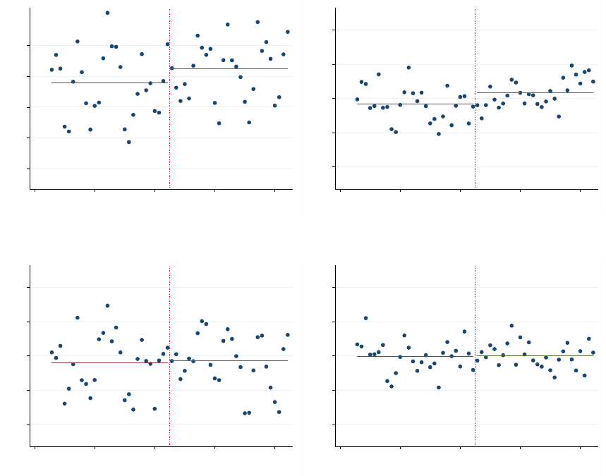
Figure 5: Bargaining Success Rates

.44 .45 .46 .47 .48

Success Rate

22apr2016 06may2016 20may2016 03jun2016 17jun2016

Day

(a) Desktop: Raw

−.02 −.01 0 .01 .02

Residual

22apr2016 06may2016 20may2016 03jun2016 17jun2016

Day

(b) Desktop: Residuals

.39 .4 .41 .42 .43

Success Rate

22apr2016 06may2016 20may2016 03jun2016 17jun2016

Day

−.02 −.01 0 .01 .02

Residual

22apr2016 06may2016 20may2016 03jun2016 17jun2016

Day

(d) Mobile: Residuals

Notes: Panels (a) and (c) depict scatterplots of the raw daily success rates for bargaining interactions grouped by

the date of the ﬁrst oﬀer for desktop and mobile, respectively. Panels (b) and (d) depict residuals from a linear

probability model regressing a dummy for successful bargaining on a large series of covariates (ln(ask price); category

by condition ﬁxed eﬀects; day of week, precipitation, and holiday dummies and the temperature) for desktop and

mobile, respectively. The vertical axes on both plots are scaled identically subject to a location shift.

half a percent. Two other features are apparent—ﬁrst, there is substantial variation

between days in the success rate of bargaining interactions, although this is rather

smaller when we condition on the set of controls. Second, and more importantly, it

appears that there is a positive drift in the residuals during the post period. In Section

5 we will oﬀer a simple economic explanation for this ﬁnding: buyers and sellers are

learning to communicate in the weeks following the policy change, leading to new

behavior and better outcomes.

Consistent with models (3) and (4) of Table 3, we see no evidence of change in

the likelihood that interactions are successful for buyers using the mobile platform..

We also see no positive drift in the residuals in the post period. This rationalizes our

ﬁnding for the diﬀerence in diﬀerences estimator

in models (5),(6),(7), and (8).

4.2.3 Week-Speciﬁc Treatment Eﬀects: Parallel Trends and Dynamics

Next, we estimate a variant of (4) with week-speciﬁc eﬀects over our eight-week sample:

1(success) = β

+ Xβ

+ P β

+ Dβ

P D · 1(week t)β

C,t

+ ε. (6)

We are interested in this model for two reasons. First, the divergence in the residualized

scatterplots for desktop, Figure 5(b), and mobile, Figure 5(d), in the post-treatment

period suggest that the eﬀect of communication on bargaining is not immediate but

delayed. Estimating week-speciﬁc eﬀects will allow us to characterize these dynamics.

Second, following Autor (2003), estimating week-speciﬁc eﬀects in the pre-period

allows a partial test of the parallel trends assumption. If estimated week-speciﬁc

eﬀects in the pre-period are signiﬁcant, this would violate Granger causality—that is,

the eﬀect would precede the cause, marking a failure of our identifying assumptions.

Results are depicted in Figure 6. We normalize the eﬀect for week zero (just before

the policy change) to zero. In the pre-period, our test of the joint signiﬁcance of the

coeﬃcients fails to reject with a F-statistic of 0.11 (and an associated critical

value

of 0.9550). Therefore, we ﬁnd neither a violation of the parallel trends assumption nor

of Granger causality for our sample. Furthermore, the model permits us to interpret

the positive drift in the post period from Figure 5(b) as a time-variant eﬀect of

communication. Despite almost instantaneous adoption, it took several weeks for the

eﬀects to be fully seen in the probability of bargaining success—this is perhaps not

surprising, as conventions for communication may have taken some time to stabilize.

We investigate this further with the content of the messages in Section 5.

4.3 Additional Speciﬁcations and Outcomes

Next, we summarize results from additional speciﬁcations, all of which are discussed

in more detail in the Appendix.

We are interested in the eﬀect of communication on other bargaining outcomes

besides breakdown, especially in the hope that this might help us understand mecha-

In Appendix 1 we estimate week-speciﬁc eﬀects for the longer sample and show that the eﬀect of

communication on bargaining success stabilized and was consistent after week ﬁve.

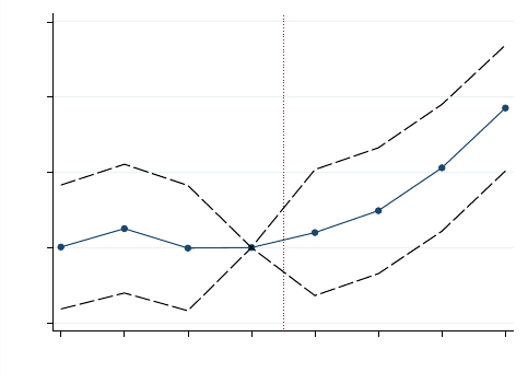
Figure 6: Week-Speciﬁc Eﬀects

−.005 0 .005 .01 .015

Estimated Effect on Success Rate

−3 −2 −1 0 1 2 3 4

Week

Notes: This ﬁgure depicts week-speciﬁc eﬀects using the diﬀ-in-diﬀ approach with the main sample, 4 weeks before

and 4 weeks after the policy change. The omitted coeﬃcient (normalized to zero) is the week just prior to the change.

Dashed lines represent a 95% conﬁdence interval with heteroskedacticity-robust standard errors clustered by seller.

nisms and distributional consequences. With the caveat of limited power, we document

our eﬀorts in Appendix B. We ﬁnd no statistically signiﬁcant eﬀects on the number of

rounds or the ﬁrst oﬀer, but we do see a strong negative eﬀect on the agreed-upon

price. Examining this more closely, we condition on who made the ﬁnal (accepted)

oﬀer in that sample, and ﬁnd suggestive evidence that bargainers are successfully

using messages to not only close the deal, but also to obtain more of the surplus.

In addition, in Appendix C we investigate heterogeneous treatment eﬀects across

asking price ranges and categories. Here our limited power is binding, however we ﬁnd

suggestive evidence that the eﬀects are somewhat larger at lower price ranges (however,

this is substantially ﬂattened when we consider proportional eﬀects, as success rates

are much lower for higher asking price products).

Also, in Appendix D we consider robustness checks along two dimensions: ﬁrst,

the window used to construct the estimation sample and second, the inclusion of seller

ﬁxed eﬀects. Both are supportive of the results of Table 3. We note that shortening

the sample makes the eﬀects no longer statistically signiﬁcant, as one might intuit

from Figure 6; that in extending it, the upward trend in Figure 6 stabilizes, and that

seller ﬁxed eﬀects somewhat attenuate the result (from 0.0773 to 0.0561).

5 Evidence of Learning from Text Analysis

In Section 4, we found a positive and signiﬁcant relationship between bargaining

eﬃciency and messaging. Moreover, by analyzing the week-speciﬁc eﬀects of messaging,

we observed that it took time for the full eﬀect of communication to materialize. In

this section, we explore the messages themselves in order to oﬀer a plausible economic

story for the strengthening relationship between messaging and bargaining success.

We compute the change in messaging content across weeks for both buyers and

sellers, and are able to uncover some compelling patterns in messaging content.

Namely, we ﬁnd that messages sent by repeat sellers, or sellers who are sending

multiple messages in our sample, are becoming more similar in content as the weeks

pass. We additionally ﬁnd convergent patterns in seller messages: speciﬁcally, the rate

at which seller messages are changing is decreasing. These trends in seller messages are

consistent with experience-based learning in which sellers adopt messaging strategies

over time. We do not ﬁnd similar results for buyers, where there are far fewer who are

sending multiple messages in our sample.

5.1 Messaging Data

We have 248,722 messages of buyer and seller interactions for the ten-week period

succeeding the introduction of messaging beginning on May 25, 2016.

We process

these messages through the following steps: First, we identify and keep only the

messages sent in German in order to maintain a common corpus of words for our

analysis; this makes up the vast majority (81.1 percent) of our dataset with the next

most common language being English (which accounts for 6.4 percent of the messages).

Second, the lower-cased messages are stripped of non-alphabetic characters, urls, extra

spaces, and a list of common stop words—these are words such as “and” and “the”

that provide little meaning in our messages. We then apply NLTK’s German Snowball

Stemmer (Bird et al. (2009)) to the tokens (ie. words) in each message so that they are

transformed to their original stems. For instance, the word “angeboten” (“oﬀered”) is

minimized to “angebot” (“oﬀer”). This step is common practice in natural language

processing and allows us to consider eﬀectively synonymous words as the same word.

Our textual analysis starts two days after the change due to low take up on May 23-24, 2016.

Please refer to Appendix Section E2 for a more detailed discussion of the construction of our

messaging dataset, including a description of the list of stop words we remove from our dataset.

Table 4: Buyer and Seller Messaging Characteristics Based on Experience

Number of Messages Unique Individuals Average Message Length Success Frequency

Buyer

All Messages 93576 76415 9.293 0.309

One Message 64648 64648 9.250 0.339

Two - Four Messages 25595 11271 9.379 0.244

Five+ Messages 3333 496 9.475 0.240

Seller

All Messages 116081 60076 8.513 0.228

One Message 40350 40350 8.218 0.243

Two - Four Messages 40541 16375 8.561 0.213

Five+ Messages 35190 3351 8.796 0.227

Notes: In the ﬁrst column messages are split based on whether the message’s corresponding buyer or seller sent one,

two to four, or ﬁve plus messages. Average message length refers to the average number of tokens in each message for

that group. Success is deﬁned by whether that message ends in a sale.

The ﬁnal reduced dataset amounts to 209,658 messages split into 93,577 buyer

messages and 116,081 seller messages. Table 4 provides descriptive statistics for buyer

and seller messages split by experience level, which we deﬁne as the total count of

messages sent by that seller or buyer over the ten-week period. Here we see that

buyers tend to be “short-run” players, with only 496 buyers sending ﬁve or more

messages. In contrast, individual sellers are more persistent in our dataset—there are

3,351 who are sending ﬁve or more messages.

Next, Table 5 depicts the ten most common tokens for buyers and sellers. Here,

sellers messages appear to be slightly more negative in messaging content as “not”

is the second most common word; additionally, “unfortunately” is the eighth most

frequent token to appear in seller messages. For a more thorough description of the

messages in our dataset, see Appendix Section E.

5.2 Empirical Challenges and Methods

Representing textual data constitutes a unique and increasingly common challenge

in empirical research. In order to analyze seller and buyer messages, we must ﬁrst

construct a measure for the content of each message.

To do this, we split each message into a series of bigrams, a two-word pairing

formed from consecutive words. For example, message

as “this is my last oﬀer”

would be broken up into the parts: [“this is,” “is my,” “my last,” and “last oﬀer”].

Splitting the messages into bigrams, rather than single-word tokens, allows us to

Table 5: Buyer and Seller Most Common Tokens

Rank Buyer Token Translation Frequency Seller Token Translation Frequency

1 Hallo Hello 0.031 Nicht Not 0.032

2 Wurd Would 0.030 Hallo Hello 0.024

3 Gruss Greeting 0.025 Gruss Greeting 0.023

4 Versand Shipping 0.018 Preis Price 0.021

5 Nicht Not 0.016 Euro Euro 0.020

6 Euro Euro 0.015 Versand Shipping 0.016

7 Mfg Kind regards 0.011 Leid Unfortunately 0.015

8 Dank Thanks 0.011 Dank Thanks 0.013

9 Kauf Purchase 0.010 Schon Beautiful 0.012

10 Preis Price 0.010 Mfg Kind regards 0.011

Notes: This table reports the frequency of the ten most common tokens in our processed dataset for buyers and sellers.

Tokens are translated to English for readability.

simplify each message while still incorporating some level of context in our textual

analysis. An example of this are the words “screw” and “you,” put together “screw

you” has a much stronger meaning than the two words apart.

Next, we collapse our data into what is known as a “bag-of-words,” or in our

case, a “bag-of-bigrams,” where each message is a row and each bigram a column.

This exercise is frequently used in natural language processing (see Gentzkow et al.

(2019a)); however, as analyzing textual data is still relatively new to economics, we

will detail what this means below.

Our bag-of-bigrams is in the form of the matrix

, where element

i,mj

corresponds

to the number of counts for phrase

in message

for group

, ie. some group of buyers

or sellers.

is a high dimensional matrix. For instance,

for all seller messages

in our dataset makes up a 116,081-by-287,241 matrix accounting for 116,081 seller

messages and the 287,241 distinct bigrams that appear in these messages. Similarly,

for buyer messages forms a matrix with dimensions 93,577-by-331,904.

We are interested in changes in messaging content at the weekly level: Thus, we

collapse

is a ten-by-

matrix with each row corresponding to a week

in our ten-week sample and

representing the number of distinct bigrams sent by

group

. Element

i,wj

then equates to the number of times phrase

appears in the

messages sent during week w by group i.

Finally, we take vector

from row

and compute the cosine distance

between

and all rows in

. The cosine distance between vector

and

given by

1 −

· v

||v

, (7)

where · represents the dot product and |v

| is the `

norm.

The cosine distance measures one minus the cosine of the angle between

and

and is a standard method for computing text dissimilarity. The normalizing term

in the denominator of

(7)

is desirable in our case as it scales the distance between

the two vectors by each vector’s length. This is essential in our context as the sum

of bigram counts varies week from week due to changes in the take-up of messaging,

holidays, etc. Finally, the cosine distance is our metric of choice as it supplies an

intuitive measure of the distance between bigram counts across weeks. Since our

vectors are by construction composed of nonnegative values, the cosine distance in

this case will always be in the range [0

Here, two weeks with orthogonal vectors

will have a cosine distance of 1, whereas the cosine distance will approach 0 as the

two vectors get more similar in counts.

Finally, in order to clearly present the cosine distances across each pairing of

weeks, we construct a ten-by-ten matrix of cosine distances with the

th element

corresponding to the cosine distance between the vector of bigram counts in week

and the vector of bigram counts in week w

5.3 Dynamics of Communication by Experience

In Figure 7, we present our results through a heat map depicting the cosine distances

between the bigram counts across weeks for buyers, Panel (a), and sellers, Panel

(b). The colors indicate cosine distances in which the lighter boxes convey greater

diﬀerences in messaging content, while the messages get more similar as the boxes get

darker.

In Panel (a) of Figure 7, the cosine distances between buyer messages is stable

across our ten-week period; we can see this as all the boxes in the heat map appear to

be similar shades of blue. Table 4 oﬀers a plausible explanation for this consistency in

buyer messages across weeks: There are few buyers in our sample sending multiple

messages. Speciﬁcally, only 3,333 messages are sent from buyers whose total message

count is ﬁve or more. In contrast, 35,190 messages are sent by sellers with ﬁve or more

messages. Due to the lack of repeat buyers, any changes in Panel (a) are presumably

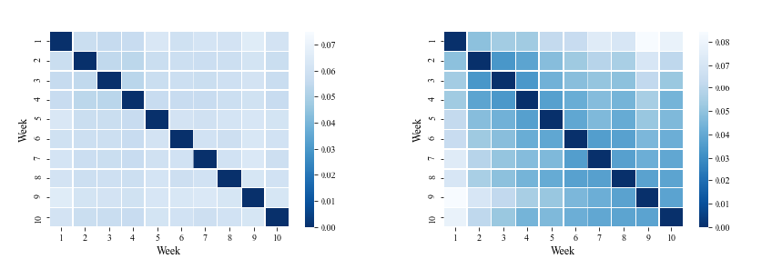
Figure 7: Cosine Distance of Buyer and Seller Messages by Week following the

Introduction of Messaging

(a) Buyer (b) Seller

Notes: This ﬁgure presents the cosine distance of the bigram counts in the messages between each of the ten weeks

following May 25, 2016, for buyers, in Panel (a), and sellers, in Panel (b).

due to noise and week-eﬀects. For instance, we observe diﬀerential usage of the word

“urlaub” or “vacation” in our sample. Buyer messages include “vacation” 61 times

during the week of July 20th, while they only mention “vacation” 21 times during the

ﬁrst week of our sample (May 25 – 31).

Panel (b) of Figure 7 portrays starkly diﬀerent results; here, there are clearly

changes in content across sellers messages from week to week as made evident due to

the patterns of color occurring in seller messages. Still, it is challenging to discern

exactly how seller messages are transforming. In order to amend this, there are two

ways in which we can more intuitively decipher the patterns presented in the heat

maps. First, we can more closely observe the bottom gradient of the heat maps, where

we are comparing the diﬀerences in messaging content between week w and week 10.

Second, we can plot the oﬀ-diagonals of the heat maps in order to see the rate of

change in message content. The former will tell us whether the content of the text is

changing systematically, where the latter will tell us whether it is convergent. That is,

if the rate of change is decreasing, we take this as evidence of the convex pattern that

is signature of models of learning and information: that our ﬁrst data points teach us

more than those that follow.

Figure 8 depicts a plot of the the cosine distances between week

and week ten

(the bottom gradient) for buyers and sellers. In this ﬁgure, we also depict the results

for (nested) subsamples with diﬀerent experience levels, where we deﬁne experience by

the number of messages sent by that seller/buyer over our entire sample. Separating

by experience level will allow us to isolate the sellers for whom we are more likely to

observe patterns of learning. The scale of each plot is normalized to 1 in the last week;

we do this because sampling variation, which is more salient as we restrict the sample

size, biases the cosine distance measure upwards and makes levels uninterpretable.

Note also that the scales of panels (a) and (b) are diﬀerent.

Panel (a) depicts the diﬀerences in messages between week

and week 10 for

buyers. The line for “All” includes all buyers, and corresponds directly to the values

in the bottom row of the heat map in panel (a) of Figure 7. For buyers with one, two,

or three or more messages, the cosine distance does not appear to be changing. For

buyers with four, ﬁve, and six or more messages, the cosine distance is decreasing over

time, but this is obscured by sampling variation due to the small number of buyers in

these sets.

In Panel (b), we again observe sharply diﬀerent results for sellers. Here again, the

line for “All” includes all sellers, and corresponds directly to the values in the bottom

row of the heat map in panel (b) of Figure 7. For all samples, we see that as the

weeks get closer to week 10, seller messages are increasingly more similar in content

to the messages from this last week. Note also that the change is more pronounced

among more experienced sellers. For instance, we see the sharpest trend for sellers

that sent 6 or more messages, where there is a substantial diﬀerence in the cosine

distance between the set of week 1 and 10 messages and the set of week 9 and 10

messages. These patterns suggest that as the weeks pass, sellers may be adopting new

messaging strategies; moreover, it appears that repeat sellers are driving the changes

in Figure 7.

So far, we have established that repeat sellers’ messaging strategies are changing as

they accumulate experience. We would like to ask whether, in addition, the changes

are convergent, i.e. whether they represent a pattern that reﬂects learning. To do this,

we plot the cosine distance across diﬀerent periods of the same length to see whether

the diﬀerences in message content are decreasing at a slower or faster rate over time.

The objects we are depicting correspond to the oﬀ-diagonal elements of the heat map

in Figure 7. The diﬀerent oﬀ-diagonals represent diﬀerences over varying lengths of

See Appendix Figure A-6 for the non-normalized version.

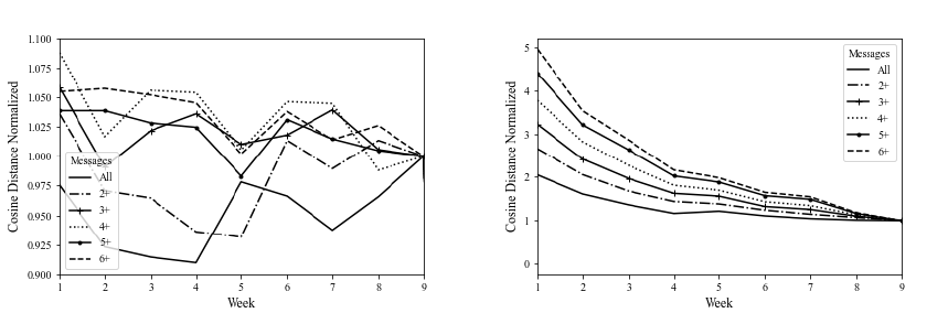
Figure 8: The Bottom Gradient for Buyers and Sellers with Diﬀerent Experience

Levels

(a) Buyer (b) Seller

Notes: This ﬁgure presents the cosine distance between the messages sent in weeks x and 10 for buyers, Panel (a),

and sellers, Panel (b). The cosine distance is scaled by the distance between week 9 and week 10 messages. Each

panel is cut by groups, where All includes our entire sample of buyers/sellers, 2+ indicates our sample of messages

sent by buyers/sellers who sent 2 or more messages, 3+ from our sample of messages sent by buyers/sellers who sent

3 or more messages, and so on.

time; we depict them all because we are concerned that high-frequency diﬀerences

may exaggerate the ratio of noise to signal.

Figure 9, plots the oﬀ-diagonals for all buyers, Panel (a), and sellers, Panel (b). In

this plot, ∆

for week

corresponds to the cosine distance in messages between week

and week

w − x.

As suspected, Panel (c) portrays a noisy plot with no obvious

patterns in buyer messages; on the other hand, there appears to be a downward trend

in the ∆

’s in Panel (d). Thus, while seller messages are becoming more similar over

time, they do so at a declining rate.

Figure 9 depicts the oﬀ-diagonals corresponding to the “All” groups of Figure 8,

but from the latter we saw that repeat sellers are changing their messaging content

more than transient ones. So, in Figure 10 we reproduces the same exercise for sellers

who sent 5 or more messages in our ten-week period. As a reference point, the heat

map for this group of sellers is depicted in Panel (a). Already, we see starker patterns

in the change in message content across weeks. Panel (b) presents the oﬀ-diagonal

plot for this group of sellers. Again, the patterns that previously emerged for our

entire dataset of sellers become much more explicit when we restrict our analysis to

repeat sellers. For instance, from ∆5 in Panel (b) we can see that sellers’ messages

between weeks 8 and 3 are more similar than in comparison to the messages for weeks

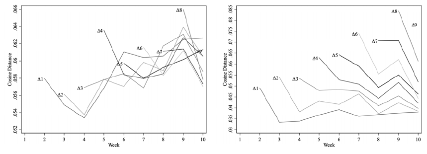
Figure 9: Oﬀ-Diagonals for Buyers and Sellers

(a) Buyer (b) Seller

Notes: This ﬁgure displays the change in cosine distance of bigram counts in the messages for diﬀerent periods of

time following May 25, 2016, separately for buyers, in Panel (a), and sellers, in Panel (b). ∆x for week w indicates

the cosine distance between week w and week w − x.

7 and 2 and weeks 6 and 1. Or in other words, as repeat sellers learn to use similar

messaging strategies over time, they are doing so at a declining rate as the weeks pass.

This convergent path in which sellers are changing their messaging content faster in

the beginning weeks following the messaging intervention, and then more slowly as

time goes by, is consistent with experienced sellers learning how to use messages to

facilitate transactions.

Most importantly, these results oﬀer a simple explanation for the dynamics seen

in Section 4.2.3, where we ﬁnd a time-variant eﬀect of communication on bargaining

success that stabilizes following week ﬁve.

Further evidence is oﬀered in Figure A-4 of the Appendix where we have included

the heat maps and oﬀ-diagonal plots for sellers who sent two, three, and four or more

messages. In addition, Figure A-5 in the Appendix presents the results for both sellers

and buyers who appear only once in our dataset. Here, the eﬀects presented above

are completely attenuated when looking at this group of sellers, further providing

evidence that these patterns of convergence are due to changes in messaging content

by experienced sellers.

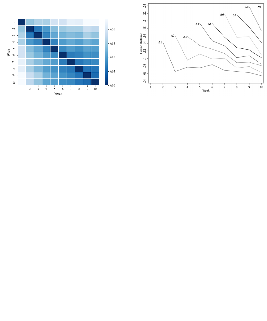
Figure 10: Convergence Among Sellers with Five or More Messages

(a) 5+ Messages (b) 5+ Messages

Notes: Panel (a) depicts the heat map representing the cosine distance of the bigram counts in the messages for each

pairing of weeks following May 25, 2016 for sellers that sent ﬁve or more messages. Panel (b) plots the oﬀ-diagonals

of the heat map from (a). ∆x for week w indicates the cosine distance between week w and week w − x.

6 Message Experience Predicts Success

In Section 4.2.3, we found a time-variant eﬀect of communication on the success rate

of bargaining; namely, it took several weeks for the full eﬀect on the success rate

to manifest. Similarly, the results from Section 5.3 indicate that seller messages are

changing over time, and that they are doing so in a convergent pattern.

Given these ﬁndings, the natural next question is whether there exists a relationship

between the change in messaging content and bargaining success. Here, we are

motivated by the bottom gradient trends in Panel (b) of Figure 8. This ﬁgure shows

that seller messages are becoming more similar as the weeks approach week 10.

To explore whether these changes are associated with shifts in the seller success

rate, we calculated the cosine similarity between each message and the aggregated set

of bigram counts from the messages sent by sellers in week 10. We regress message

success, a binary variable representing whether that seller’s message ended in a sale,

onto this cosine similarity measure.

In this analysis we exclude a small set of sellers who send more than 20 messages. We do

this because we believe that a) they are qualitatively diﬀerent, professional sellers and b) they are

overrepresented in message-level regressions. Overall, we are dropping 217 sellers that sent 21 or

more messages; this is out of our original sample of 60

076 sellers. In Appendix Section 4 we report

variations, including using all sellers and the set of sellers that sent fewer than 11 messages.

Table 6: The Relationship Between Message Success and Cosine Similarity

(1) (2) (3)

Sim(m, week 10) 0.0661

∗

0.0559

∗

0.0490

(0.0226) (0.0227) (0.0428)

Message Length 0.0013

∗

0.0003

(0.0002) (0.0005)

N 101931 101931 62217

Controls X X X

Seller FE X

Notes: This table presents our results on message success and a measure of message experience. Sim(m, week 10)

is the cosine similarity between a message and the set of week 10 messages excluding sellers who sent more than 21

messages. All models include our main set of controls: time trend; ln(ask price); category by condition ﬁxed eﬀects;

day of week, precipitation, holiday dummies, and the temperature. Likewise, all models drop sellers sending more

than 20 messages. Model (3) includes seller ﬁxed eﬀects. Robust standard errors are reported in parentheses and

∗

denotes statistical signiﬁcance at α = 0.05.

Table 6 presents our results. In all speciﬁcations we include the same set of controls

as documented in Section 3.2. Finally, Models (2) and (3) also control for message

length, as measured by the number of tokens in the processed message. Model (3)

includes seller ﬁxed eﬀects.

In Model (1), we ﬁnd a statistically signiﬁcant eﬀect that going from a completely

orthogonal message to a message containing the set of week 10 messages is associated

with an increase in the probability of success by 6

61 percentage points. In Model (2),

we further ﬁnd that message length has a positive, but economically small, relationship

with the success rate. Finally, our result is no longer statistically signiﬁcant, in Model

(3), when including seller ﬁxed eﬀects. We have only 3,134 sellers sending more

than ﬁve messages, but fewer than 21; as a result, we lose a considerable amount

of power in our estimates when restricting attention to within-seller variation. Still,

the relationship between our cosine similarity measures and message success remains

positive.

Altogether, Table 6 points to a positive correlation between the probability of

message success and the similarity between the message and the set of week 10 seller

messages. Notably, the point estimates from this table are similar in magnitude to

the point-estimates from Table 3, where we found that among our treatment group,

interactions that involved messages were 7.73 percentage points more likely to end in

success.

A limitation of our approach is that we have not been able to address the di-

rect mechanism in which messages contribute to higher rates of bargaining success.

While we cannot provide causal evidence on this front, we implement a distributed

multinomial model from Taddy (2015) in Appendix Section F. Here we consider the

relationship between the bigrams included in seller messages and the message number

sent by that seller, a measure of seller experience, which we have found to be related

to message success. This analysis attempts to further understand how seller messaging

content is changing, and through this descriptive exercise, we suggest some potential

strategies that sellers may be implementing.

Table A-7 then presents the bigrams, both in English and the original German,

that are the most and least predictive of seller experience, conditional on a set of

controls. In addition, we use the bigram coeﬃcients estimated from our model to

compute message experience scores; here, a higher score indicates a message associated

with higher levels of seller experience. Table A-8 then shows the messages with the

highest experience scores, while Table A-9 includes the messages with the lowest

scores.

Among the messages that are most correlated with experience, we see an emphasis

on costs, especially those which may not be salient to buyers, such as the eBay

commission.

This is consistent with prior work highlighting the eﬀectiveness of

cost rationales originally raised by Kahneman et al. (1986), and re-emphasized in a

bargaining setting by Lee and Ames (2017). The latter work contrasts cost rationales

with disparagement rationales, showing the latter to be ineﬀective. With respect to

this, our focus on seller messages obviates disparagement, however we do observe that,

among those messages least predictive of experience, arguments about the quality of

the product are common. We also see that where those most correlated with experience

are restrained, polite, and precise, those less so tend to use more eﬀusive language,

which is reminiscent of the ﬁnding, by Jeong et al. (2019), that warm language may

be counterproductive in negotiations.

The price that the buyer pays is not received by the seller. Instead, the platform takes a “ﬁnal

value fee” in the range of 10%. Buyers who have never been on the other side of the marketplace

might easily be unaware of this fact.

7 Discussion

In this paper we exploited a natural experiment in the availability of text messaging

in bargaining to study the role of cheap-talk communication in avoiding bargaining

breakdown. We found a statistically and economically signiﬁcant eﬀect: bargainers

who used the messaging feature were on average eight percentage points more likely

to transact. Against the sample average success rate of forty-four percent, this implies

a fourteen percent reduction in the likelihood of bargaining breakdown.

We are unaware of any prior empirical work on communication in bargaining,

however our results are consistent with a line of thought from the experimental and

theoretical literature that suggests a role for behavioral considerations in bargaining.

These papers have found that players communicate “too much” to be rationalized by

rational models of cheap talk, and oﬀer suggestive evidence that communication allows

bargainers to outperform theoretical upper bounds to bargaining eﬃciency in the

canonical, rational model with incomplete information. From the perspective of the

literature, our results cast a positive light on eﬀorts to test models that incorporate

behavioral components to understand the role of communication (Miettinen, 2013;

Dufwenberg et al., 2017).

From a market design perspective, our results suggest that communication has an

important role to play in fostering transactions. However, this analysis has sidestepped

a competing concern of platforms: that allowing communication may enable parties

to take their transactions oﬀ the platform to avoid fees. Conspicuously, among the

three largest online platforms that allow bargaining, Amazon both charges the highest

transaction fee and does not facilitate communication between buyers and sellers.

While we have no data on such oﬀ-platform transactions and cannot speak to their

frequency, we do note that they would appear as bargaining failure in our dataset.

Therefore, if communication is facilitating bargainers taking transactions oﬄine, our

results can be interpreted as net of any such eﬀect, and in that sense a conservative

estimate of the eﬀect of communication on breakdown.

Our ﬁnding that communication plays an important role in bargaining raises at

least as many questions as it answers, and we believe this is an important area for

continued work. A promising direction that we have broached but not exhausted is

to use developments in natural language processing and text analysis to study the

content of what people say, above and beyond the fact that they say something. These

questions have already been raised in experimental settings (see Lee and Ames (2017)

for a recent contribution to, and summary of, this literature in social psychology).

The availability of data from online bargaining marketplaces is an opportunity to see

them in the ﬁeld and directly link them to economic outcomes. Understanding how to

improve bargaining outcomes is among the most central questions in economics, and

also among the questions on which we have made the least progress, in part due to

a lack of empirical work using data from real market interactions. Our paper tries

to ﬁll some of that gap, and our results highlight the importance of communication

in bargaining. As Farrell and Gibbons (1989) write, “the economic importance of

costless, nonveriﬁable, informal communication is much greater than its role in the

literature suggests.” Our result documents empirically that this remains true today.

References

Angrist, Joshua D., Guido W. Imbens, and Donald B. Rubin

, “Identiﬁcation of Causal

Eﬀects Using Instrumental Variables,” Journal of the American Statistical Association, 1996, 91

(434), 444–455.

Autor, David

, “Outsourcing at Will: The Contribution of Unjust Dismissal Doctrine to the Growth

of Employment Outsourcing,” Journal of Labor Economics, 2003, 21 (1), 1–42.

Awaya, Yu and Vijay Krishna

, “On Communication and Collusion,” American Economic Review,

2015, 106 (2), 285–315.

Ayres, Ian and Barry Nalebuﬀ

, “Common Knowledge as a Barrier to Negotiation,” UCLA Law

Review, 1997, 44 (6), 1631–1660.

Backus, Matthew, Tom Blake, and Steven Tadelis

, “On the Empirical Content of Cheap-Talk

Signaling: An Application to Bargaining,” The Journal of Political Economy, 2019, 127 (4),

1599–1628.

, , Bradley Larsen, and Steven Tadelis

, “Sequential Bargaining in the Field: Evidence

from Millions of Online Bargaining Interactions,” Quarterly Journal of Economics, 2020, 135 (3),

1319–1361.

Belkin, Liuba Y, Terri R Kurtzberg, and Charles E Naquin

, “Signaling Dominance in Online

Negotiations: The Role of Aﬀective Tone,” Negotiation and Conﬂict Management Research, 2013,

6 (4), 285–304.

Bird, Steve, Edward Loper, and Ewan Klein

, in “Natural Language Processing with Python,”

O’Reilly Media Inc., 2009.

Blume, Andreas and Andreas Ortmann

, “The Eﬀects of Costless Pre-Play Communication:

Experimental Evidence from Games with Pareto-Ranked Equilibria,” Journal of Economic Theory,

2007, 132 (1), 274–290.

Bolton, Gary E., Kalyan Chatterjee, and Kathleen L. McGinn

, “How Communication Links

Inﬂuence Coalition Bargaining: A Laboratory Investigation,” Management Science, 2003, 49 (5),

583–598.

Brown, Jennifer Gerarda and Ian Ayres

, “Economic Rationales for Mediation,” Virginia Law

Review, 1994, 80 (2), 323–402.

Cabral, Luis and J´ozsef S´akovics

, “Must Sell,” Journal of Econoomics and Management Strategy,

1995, 4 (1), 55–68.

Cai, Hongbin and Joseph Tao-Yi Wang

, “Overcommunication in Strategic Information Trans-

mission Games,” Games and Economic Behavior, 2006, 56, 7–36.

Card, David and Gordon Dahl

, “Bargaining and the Role of Expert Agents: An Empirical Study

of Final-Oﬀer Arbitration,” The Review of Economics and Statistics, 2012, 94 (1), 116–132.

Charness, Gary

, Communication in Bargaining Experiments, Vol. Oxford Handbook of Economic

Conﬂict Resolution, Oxford University Press,

and Martin Dufwenberg

, “Promises and Partnership,” Econometrica, 2006, 74 (6), 1579–1601.

and , “Participation,” American Economic Review, 2011, 101, 1211–1237.

Clark, Robert and Jean-Fran¸cois Houde

, “The Eﬀect of Explicit Communication on Pricing:

Evidence from the Collapse of a Gasoline Cartel,” The Journal of Industrial Economics, 2014, 62

(2), 191–228.

Coﬀman, Lucas and Paul Niehaus

, “Pathways of Persuasion,” Games and Economic Behavior,

2020, 124, 239–253.

Cooper, David J. and Kai-Uwe K¨uhn

, “Commuication, Renegotiation, and the Scope for

Collusion,” American Economic Journal: Microeconomics, 2014, 6 (2), 247–278.

Cooper, Russel, Douglas V. DeJong, Robert Forsythe, and Thomas W. Ross

, “Commu-

nication in Coordination Games,” Quarterly Journal of Economics, 1992, 107 (2), 739–771.

Crawford, Vincent P.

, “A Theory of Disagreemnt in Bargaining,” Econometrica, 1982, 50 (3),

607–637.

, “Explicit Communication and Bargaining Outcomes,” American Economic Review, 1990, 80 (2),

213–219.

and Joel Sobel

, “Strategic Information Transmission,” Econometrica, 1982, 50 (6), 1431–1451.

, Miguel A. Costa-Gomes, and Nagore Iriberri

, “Structural Models of Nonequilibrium

Strategic Thinking: Theory, Evidence, and Applications,” Journal of Economic Literature, 2013,

51 (1), 5–62.

Doraszelski, Ulrich, Gregory Lewis, and Ariel Pakes

, “Just Starting Out: Learning and Price

Competition in a New Market,” 2017. accepted, American Economic Review.

Dufwenberg, Martin, Maro˘s Serv´atka, and Radovan Vadovi˘c

, “Honesty and Informal Agree-

ments,” Games and Economic Behavior, 2017, 102, 269–285.

Ellingsen, Tore and Robert

Ostling

, “When Does Communication Improve Coordination?,”

American Economic Review, 2010, 100, 1695–1724.

Ert, Eyal, Stephanie Creary, and Max H. Bazerman

, “Cynicism in Negotiation: When

Communication Increases Buyers’ Skepticism,” Judgement and Decision Making, 2014, 9 (3),

191–198.

Farrell, Joseph and Robert Gibbons

, “Cheap Talk Can Matter in Bargaining,” Journal of

Economic Theory, 1989, 48 (1), 221–237.

Fey, Mark and Kristopher W. Ramsay

, “When is Shuttle Diplomacy Worth the Commute?

Information Sharing through Mediation,” World Politics, 2010, 62 (4), 529–560.

Gentzkow, Matthew, Bryan Kelly, and Matt Taddy

, “Text as Data,” Journal of Economic

Literature, 2019, 57 (3), 535–574.

, Jesse M Shapiro, and Matt Taddy

, “Measuring Group Diﬀerences in High-dimensional

Choices: Method and Application to Congressional Speech,” Econometrica, 2019, 87 (4), 1307–

1340.

Gibson, Ranja, Carmen Tanner, and Alexander Wagner

, “Preferences for Truthfulness:

Heterogeneity Among and Within Individuals,” American Economic Review, 2013, 103 (1),

532–548.

Gizatulina, Alia and Olga Gorelkina

, “Selling ‘Money’ on eBay: A Field Study of Surplus

Division,” 2017. Working Paper.

Gneezy, Uri

, “Deception: The Role of Consequences,” The American Economic Review, 2005, 95

(1), 384–394.

Goltsman, Maria, Johannes H¨orner, Gregory Pavlov, and Francesco Squintani

, “Media-

tion, Arbitration, and Negotiation,” Journal of Economic Theory, 2009, 144 (4), 1397–1420.

Harrington, Joseph E. and Lixin Ye

, “Collusion through Coordination of Announcements,” The

Journal of Industrial Economics, 2019, 67 (2), 209–241.

Hine, Michael J, Steven A Murphy, Michael Weber, and Gregory Kersten

, “The Role of

Emotion and Language in Dyadic E-Negotiations,” Group Decision and Negotiation, 2009, 18 (3),

193–211.

H¨orner, Johannes, Massimo Morelli, and Francesco Squintani

, “Mediation and Peace,”

Review of Economic Studies, 2015, 82 (4), 1483–1501.

Jeong, Martha, Julia Minson, Michael Yeomans, and Francesca Gino

, “Communicating

with Warmth in Distributive Negotiations is Surprisingly Counterproductive,” Management Science,

2019, 65 (12), 5813–5837.

Kahneman, Daniel, Jack L. Knetsch, and Richard Thaler

, “Fairness as a Constraint on

Proﬁt Seeking: Entitlemenets in the Market,” American Economic Review, 1986, 76 (4), 728–741.

Kopelman, Shirli, Ashleigh Shelby Rosette, and Leigh Thompson

, “The Three Faces of Eve:

Strategic Displays of Positive, Negative, and Neutral Emotions in Negotiations,” Organizational

Behavior and Human Decision Processes, 2006, 99 (1), 81–101.

Lee, Alice J. and Daniel R. Ames

, ““I Can’t Pay More” Versus “It’s not Worth More”: Divergent

Eﬀects of Constraint and Disparagement Rationales in Negotiations,” Organizational Behavior

and Human Decision Processes, 2017, 141, 16–28.

Loertscher, Simon and Leslie M. Marx

, “Countervailing Power, Integration, and Investment

under Incomplete Information,” 2020. Working Paper.

McGinn, Kathleen L., Katherine L. Milkman, and Markus N¨oth

, “Walking the Talk in

Multiparty Negotiation: An Experimental Investigation,” Journal of Economic Psychology, 2012,

33 (1), 278–291.

, Leigh Thompson, and Max H. Bazerman

, “Dyadic Processes of Disclosure and Reciprocity

in Bargaining with Communication,” Journal of Behavioral Decision Making, 2003, 16, 17–34.

Menzio, Guido

, “A Theory of Partially Directed Search,” Journal of Political Economy, 2007, 115

(5), 748–769.

Miettinen, Topi

, “Promises and Conventions – An Approach to Pre-Play Agreements,” Games

and Economic Behavior, 2013, 80, 68–84.

Myerson, Roger B and Mark A Satterthwaite

, “Eﬃcient mechanisms for bilateral trading,”

Journal of economic theory, 1983, 29 (2), 265–281.

Oberholzer-Gee, Felix and Julie Wulf

, “Alibaba’s TaoBao,” Technical Report 9-709-456, Har-

vard Business School 2009.

Radner, Roy and Andrew Schotter

, “The Sealed-Bid Mehanism: An Experimental Study,”

Journal of Economic Theory, 1989, 48 (1), 179–220.

Rubinstein, Ariel

, “Perfect Equilibrium in a Bargaining Model,” Econometrica, 1982, 50 (1),

97–110.

Taddy, Matt

, “Distributed Multinomial Regression,” The Annals of Applied Statistics, 2015, 9 (3),

1394–1414.

Valley, Kathleen, Leigh Thompson, Robert Gibbons, and Max Bazerman

, “How Commu-

nication Improves Eﬃciency in Bargaining Games,” Games and Economic Behavior, 2002, 38 (1),

127–155.

Appendices

A A Straw Man: OLS Estimates

In the absence of a natural experiment, one might have been tempted to analyze

the eﬀect of communication by regressing a dummy for success on a dummy for the

presence of a message. This will be misleading if bargainers are more likely to send

messages when an interaction is, for reasons unobservable in our set of controls, less

likely to succeed. In Table A-1 we present OLS estimates for such an analysis in a

linear probability model approach.

Note that for these results we construct the message indicator a bit diﬀerently.

(Message

∗

) is actually

(complier), the product of three dummy variables: one for

whether any message was sent, one for whether the ﬁrst oﬀer in the interaction was

made after May 23, 2016 (to rule out misclassiﬁed messages), and one for whether

the buyer is a desktop user (to rule out cases where a message was sent by the seller

but the buyer could not read it because they were on the mobile app). In models (1)

through (4) we progressively add additional controls. The coeﬃcient on

(Message

∗

)

responds most signiﬁcantly at the inclusion of ln(Asking Price), which is intuitive

because messages are more common when bargaining over more expensive goods,

recalling Table 2. However, the coeﬃcient stabilizes at a relatively slight 1.5 percentage

points, which is substantially lower than our estimated treatment-eﬀect-on-the-treated

of approximately 8. We take this to mean that the endogenous decision of whether

to send a message is strongly negatively correlated with the error term in the OLS

regressions. That is, bargainers are more likely to use messages when the chances of

success are slight for reasons unobservable to the econometrician—evidence for this

already appears in the diﬀerence between models (1) and (2), where the inclusion of

the asking price removes some of the negative bias. Recall from Table 2 that messages

are more frequently sent when the asking price is greater, which is also where the

likelihood of breakdown is greater.

Appendix-1

Table A-1: OLS Estimates

(1) (2) (3) (4) (5) (6)

1(Message) -0.0076

∗

0.0208

∗

0.0152

∗

0.0151

∗

(0.0028) (0.0027) (0.0026) (0.0026)

ln(Ask Price) -0.0827

∗

-0.0840

∗

-0.0840

∗

-0.0840

∗

-0.0840

∗

(0.0013) (0.0013) (0.0013) (0.0013) (0.0013)

Time Trend 0.0000 0.0001 0.0000 0.0000

(0.0000) (0.0000) (0.0000) (0.0000)

1(Monday) 0.0115

∗

0.0115

∗

0.0114

∗

(0.0011) (0.0011) (0.0011)

1(Tuesday) 0.0073

∗

0.0074

∗

0.0069

∗

(0.0011) (0.0011) (0.0011)

1(Wednesday) 0.0046

∗

0.0046

∗

0.0043

∗

(0.0012) (0.0012) (0.0012)

1(Thursday) 0.0022

∗

0.0023

∗

0.0022

∗

(0.0011) (0.0011) (0.0011)

1(Friday) -0.0087

∗

-0.0086

∗

-0.0088

∗

(0.0013) (0.0013) (0.0013)

1(Saturday) -0.0106

∗

-0.0106

∗

-0.0108

∗

(0.0012) (0.0012) (0.0011)

1(Precipitation) -0.0014

∗

-0.0014

∗

-0.0008

(0.0007) (0.0007) (0.0007)

1(Holiday) -0.0072

∗

-0.0072

∗

-0.0078

∗

(0.0011) (0.0011) (0.0011)

Temperature 0.0006

∗

0.0006

∗

0.0006

∗

(0.0001) (0.0001) (0.0001)

Category by Condition FE X X X X

N 3294362 3294362 3294362 3294362 3294362 3294362

Notes: This table reports OLS coeﬃcients from a linear probability model in which each observation is a bargaining

interaction and the dependent variable is a dummy for whether negotiations ended in a transaction. 1(Sunday) is

excluded. Heteroskedacticity-robust standard errors, clustered by seller, are reported in parentheses, and

∗

denotes

statistical signiﬁcance at α = 0.05.

B Alternative Outcomes

The bulk of our analysis has taken a dummy for bargaining success as the dependent

variable. We might also be interested to know how other bargaining outcomes change

with the introduction of communication. For instance, do buyers negotiate better

deals? Is bargaining prolonged?

Appendix-2

Our results for these questions are presented in Table A-2. Models (1) and (2)

consider dependent variables for which we can use the entire sample: respectively, the

number of oﬀers in the bargaining interaction and the log of the ﬁrst buyer oﬀer. We

ﬁnd no statistically signiﬁcant eﬀect on either of these outcomes. In model (3) where

we condition on bargaining success and measure the eﬀect on negotiated prices. We

ﬁnd a strong negative eﬀect. Note for models (2) and (3) that the controls include the

sellers’ asking price, so we can interpret this eﬀect as a discount. One interpretation

is that sellers have raised their asking prices, but we ﬁnd such general equilibrium

eﬀects unlikely because of the low take-up rates of the messaging feature; also, we see

no compositional changes in the prices bargained in the pre- and post periods. This

leaves two additional hypotheses: ﬁrst, that transactions that are new—that is, would

not have happened but for messaging—are on average for lower-priced products than

those that are not. This is consistent with the ﬁnding of Valley et al. (2002), as the

new transactions are on the frontier where buyer and seller valuations are close, as well

as our failure to ﬁnd an eﬀect on the buyer’s initial oﬀer. An alternative interpretation

is that the composition of goods has not changed, but buyers are taking more of the

surplus.

Next, in models (4), (5), and (6) we dive further into the question of the division

of surplus. Here, we construct subsamples deﬁned by the endogenous bargaining

sequence. Model (4) uses the asking price for the subsample where the buyer’s initial

oﬀer is accepted (recall that buyers always make the ﬁrst oﬀer). Model (5) takes the

subsample in which the buyers initial oﬀer was countered, and the seller’s counter-oﬀer

was accepted. Finally, model (6) takes the subsample in which the buyer’s initial oﬀer

was countered, then the buyer countered the seller’s counter, and the seller accepted

that counter-oﬀer. In model (4) do we ﬁnd an almost-signiﬁcant eﬀect. Moreover, the

sign changes between the models are consistent with the hypothesis that bargainers

are using messages to their own advantage. Note that the sample size shrinks fast

when conditioning on these small subsets, so it is unsurprising that we lack the power

to identify a signiﬁcant eﬀect.

Appendix-3

C Heterogeneous Eﬀects

1 Eﬀects by Price Range

Next, we present estimates of

across diﬀerent price categories in Table A-3. Our

estimates range from 8.98 to 10.44 percentage points for interactions where the asking

price is below

150, and they are substantively smaller—statistically insigniﬁcant with

point estimates ranging from 2.41 to 3.51 percentage points above $150.

While it seems as if there is a substantially larger eﬀect of communication for

interactions that involve listings with lower asking prices, we note that this relationship

ﬂattens out when we consider the baseline success rates. Interactions in the lowest-

price group (asking price less than

50) are successful 52.94 percent of the time, while

listings in highest-price group (asking prices above

250) are successful 25.54 percent

of the time. So the proportional eﬀect is rather more similar—and not statistically

distinguishable—and therefore we hesitate to draw conclusions.

2 Variation Across Categories

We next turn to category-speciﬁc estimates of

. However, we note two words of

caution: ﬁrst, because the eﬀects we are estimating are so small—from Table 3, on

the order of half a percent—splitting our sample quickly erodes power. In that spirit,

the standard errors should be interpreted with caution because a table with many

estimates implicitly suﬀers a multiple comparison problem. Similarly, the ordinal

relationships of the point estimates should be interpreted with substantial caution.

Second, we remind the reader that selection into the Best Oﬀer mechanism is

endogenous. The composition of, for instance, CDs and DVDs conditional on enabling

Best Oﬀer may be very diﬀerent than CDs and DVDs more generally. While we may

think of the latter as being rather standardized, the former may be more likely to

include box sets and out-of-print collectors editions.

Estimates are presented in Figure A-1. The dependent variable remains a dummy

for whether the bargaining ended in a transaction. Standard errors are not adjusted

for the multiple comparison problem. While we ﬁnd intuition in some of the ﬁndings,

e.g. the large eﬀect in Collectibles, others remain a puzzle, e.g. the large eﬀect in

Appendix-4

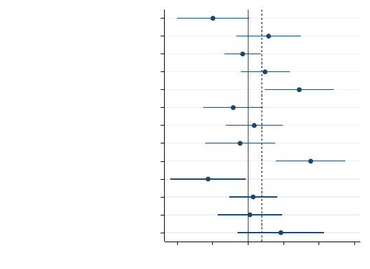
Figure A-1: Category-Speciﬁc Eﬀects

Antiques & Art

Business & Industry

Car and Motorbike: Parts

Clothing & Accessories

Collectables

Computers, Tablets & Networking

Furniture & Living

Tools

Mobile Phones

PC & Video Games

Sports

TV, Video & Audio

Watches & Jewellery

−.4 −.2 0 .2 .4 .6

Notes: This ﬁgure presents category-speciﬁc estimates for all categories in our main sample with at least one hundred

thousand interactions. The dependent variable is a dummy for whether the bargaining interaction ended in a trans-

action. All parameters of the model are estimated independently for each coeﬃcient estimate. The solid vertical line

is at zero, while the dashed vertical line is at our point estimate from Table 3 of 0.0773 for comparison.

Mobile Phones or the negative one in Antiques and Arts. For the reasons above, we

do not put much stock in these comparisons, ordinal or absolute.

D Robustness

1 Sample Window

As a simple robustness test, we check the sensitivity of our estimates to the sample

window. The main sample window is four weeks before and four weeks after the

change on May 23, 2016, depicted graphically in Figure 3. We also consider two, three,

ﬁve, and six weeks in either direction, as well as the full dataset, seven weeks before

and ten weeks after.

Table A-4 presents estimates varying the sample window. Consistent with the

ﬁnding that the eﬀect of introducing communication is not immediate, results are

weaker for the shorter windows. This also reﬂects a loss of power as we lose observations.

Extending the window for a longer time horizon, the estimates stabilize, however this

may reﬂect other changes on the website. Consistent this, we also re-create Figure 6

for the full sample, estimating week-speciﬁc eﬀects six weeks before and ten weeks

Appendix-5

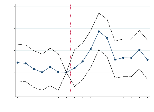
after the policy change. Estimates are presented in Figure A-2. Here it appears that

the treatment eﬀect of communication stabilizes after ﬁve weeks.

Figure A-2: Week-Speciﬁc Eﬀects—Extended Sample

−.005 0 .005 .01 .015

Estimated Effect on Success Rate

−6 −5 −4 −3 −2 −1 0 1 2 3 4 5 6 7 8 9 10

Week

Notes: This ﬁgure depicts week-speciﬁc eﬀects using the diﬀerences-in-diﬀerences approach with the extended sample

which uses seven weeks before the change and ten after. The omitted coeﬃcient (normalized to zero) is the week just

prior to the change.

2 Seller Fixed Eﬀects

Next, we consider replicating the estimates from Table 3 with seller ﬁxed eﬀects. This

is meant to address a number of concerns. Most importantly, the category ﬁxed eﬀects

that we include in our main speciﬁcation are rather coarse, and so seller-level ﬁxed

eﬀects might do a better job of controlling for product unobservables. In particular,

we are concerned that the composition of listings on which interactions are occurring

is diﬀerent in unobservable ways for the treated group and the untreated group, which

might lead us to ﬁnd spurious eﬀects.

Estimates are presented in Table A-5. We have limited ourselves to replicating only

the models with the full set of controls. We see a slight attenuation of the estimates,

but the

and

remain statistically signiﬁcant and statistically indistinguishable

from the estimates of Table 3.

Appendix-6

E Text Analysis Details

1 Message Examples

Table A-6 shows a curated set of examples messages sent with oﬀers in our data.

Messages range from the simple declaration of an oﬀer to signals of willingness-to-pay

or accept (e.g. “I do not go down”).

Some messages are meant to entice better oﬀers,

such as oﬀering bulk discounts. Some messages clarify aspects of the item (like missing

a hard drive). Still others seem like endearment and politeness, perhaps an attempt

to foster or appeal to other-regarding preferences. Therefore, messages seem to serve

a multitude of functions: cheap talk, signaling about buyer and seller characteristics,

resolving informational uncertainties about the product, endearment, and more.

2 Data Construction

The text analysis of Section 5 uses the dataset of 248,722 messages sent in the ten

weeks following May 25, 2016. This reﬂects some preliminary cleaning: messages

consisting only of numbers or spaces are excluded. Also, messages such as “please

enter your message here” (in a variety of languages), which we believe to be an artifact

of third-party software for sellers to create listings and upload them via the API, have

been manually detected and excluded.

Most of the analysis is conducted on the “processed” messaging dataset. The

processing of the messaging takes place in four steps.

First, we use a Python implementation of Google’s language detection algorithm

to classify messages by language. After this, we keep only the messages that are

detected to be in German.

2. Second, we remove all numbers, symbols, and extra spaces from each message.

Third, we remove stop words. This list of stop words comes from NLTK’s set

of German stop words. We remove “nicht” (“not”) from this list as this token

appears to be important in the context of bargaining.

Next, we stem the messages. To do this we use the NLTK’s German Snowball

Stemmer.

“MFG” is a common acronym translating to “with regards.”

Appendix-7

3 Heat Maps and their Corresponding Figures

Figure A-3 shows our heat map results and oﬀ-diagonal plots for diﬀerent cuts of

buyers based on the number of messages they sent throughout the ten week period

following the introduction of messaging on eBay Germany Best Oﬀer. As expected,

these ﬁgures are ﬁlled with noise and present no obvious patterns. Figure A-4 depicts

the same ﬁgures, but for sellers. Here, we ﬁnd that our results strengthen as we

restrict attention to experienced sellers. As a robustness check, Figure A-5 presents

the heat map ﬁgures and oﬀ-diagonal plots for buyers and sellers who only sent one

message during this time period. We ﬁnd that sellers that send only one message have

no patterns in messaging content, which further suggests that seller learning is driving

our results among experienced sellers.

Figure A-6 includes the bottom gradient results for buyers and sellers without

being scaled by the cosine distance between week 9 and week 10 messages. As seen in

Panel (a), the cosine distance for buyer messages is close to being orthogonal (near

one) for the group of buyers that sent six or more and ﬁve or more messages. One

reason we are getting this result is because we have few buyers who’ve sent multiple

messages, for instance, only 496 buyers sent ﬁve or more messages. This highlights

one weakness of our cosine distance measure, namely that it’s sensitive to the number

of messages in each sample.

As a robustness check, Figure A-7 then includes the number of messages by group

for buyers and sellers across weeks. We also include these ﬁgures scaled by the number

of messages in week 10. In this ﬁgure, there is some noise in the number of messages

by week, however, we don’t see a signiﬁcant rise in the number of messages sent by the

set of sellers with multiple messages in later weeks—such a rise would cause concern

for our main results in Section 5.3.

F An Exploration into Seller Messages

In Section 4, we presented results that suggest that sellers are learning across our

ten-week sample period; furthermore, we found that this result is driven by experienced

sellers. In this section, we implement a distributed multinomial regression model

(DMR) from Taddy (2015) that explores the relationship between seller experience

and the bigrams sent by sellers in our messaging dataset.

Appendix-8

1 Data Reduction

For this analysis, we are using the same dataset as the one discussed in Section 5.1.

Similar to Section 5.2, we construct a matrix

consisting of seller bigram counts;

recall that element

s,mj

corresponds to the number of counts for bigram

message

. Now, in order to lower the computational costs of running a regression

model, we went through of series of cleaning steps. These steps were aimed at reducing

some of the high dimensionality of our messaging dataset without loss of signiﬁcant

information—as mentioned, we have more than 280,000 bigrams in our original sample

of seller messages.

The processing steps are as follows: 1) we remove bigrams that contain less than 5

characters, 2) we remove bigrams where one of the tokens in the bigram contain only

1 character, 3) we drop all sellers that sent more than 21 messages, 4) we remove all

bigrams that are used less than 10 times across seller messages, 5) we drop bigrams

that are said by only one seller, and 6) we remove the empty rows that the previous

two steps created in matrix C

For step 3, we drop sellers that are sending more than 21 messages as we expect that

these sellers might be very diﬀerent than sellers sending between 1 and 20 messages;

for instance, these serial sellers are probably more likely to be active on diﬀerent

sites and, as a result, they might already have had experience sending messages to

buyers prior to the introduction of messaging on eBay’s Germany Best Oﬀer platform.

Second, as we are concerned about how sellers are changing messaging content from

one message to another, it makes sense for us to set bounds on the message number.

Dropping these sellers from our sample only removes 217 sellers out of our original

076. In total, these steps reduce the dimension of matrix

to be 86,879-by-8,069;

representing the 86,879 messages in our sample that contain 8,069 unique bigrams.

We construct our ﬁnal dataset by then merging a number of controls to our matrix

of bigram counts. In addition to the controls documented in Section 3.2, we add

dummies for the total number of messages sent by that seller, a variable representing

the message length—which we measure by the number of tokens in the raw message—

and the log of the oﬀer price attached to the message. We then have 242 controls

included in our analysis.

Appendix-9

2 The DMR Model

Our main variable of interest is the message number sent by that seller. Here, we

hope to further understand the bigrams that are correlated to seller experience. To do

this, we implement a distributed multinomial model from Taddy (2015). This model

was additionally used as the preferred speciﬁcation in Gentzkow et al. (2019b); in

this paper, the authors analyze congressional speeches from 1873 to 2016 in order to

estimate the trends in partisanship.

In implementing this model, we are ﬁrst assuming that our bigrams counts are

being generated by the multinomial distribution.

Speciﬁcally, the counts in each

message

are drawn by the multinomial distribution with parameters

the total number of bigrams said in message

, and probability vector

, indicating

the probability of including each bigram conditional on the controls speciﬁed in the

previous section. To compute these probability vectors, we we would then estimate

exp(ζ

)

l=1

exp(ζ

)

, where ζ

= α

+ β

+ ρ

Here, the vector

represents our set of controls for message

; additionally, message

number, our proxy for experience, is denoted by x

Rather than running a computationally intensive multinomial logistic regression,

Taddy (2015) notes that we can instead assume

∼ P ois

(

exp

[

])

where we ﬁx

ˆµ

log

(

). This allows us to run separate Poisson regressions

for each bigram.

For each Poisson regression we then estimate the coeﬃcient on message number

for bigram j by minimizing

exp(ζ

) − c

(ζ

)] + λ[

|β

| + |ρ

|].

In this equation, we include L1 regularization through the penalizing term, λ, which

reduces the number of features in our model by shrinking the coeﬃcients

and

This assumes that each bigram in a message is independently generated. While this assumption

is undoubtedly violated, assuming a multinomial distribution for text is common practice (see Taddy

(2015), Gentzkow et al. (2019a)).

Note that the coeﬃcients for our controls and message number are standardized so that they

have a standard deviation of one.

Appendix-10

toward zero. For this exercise, we selected the

that minimizes the mean out-

of-sample deviance using 10-fold cross-validation (CV).

We chose to incorporate

variable selection into our model in order to generate a more interpretable output and

to avoid over-ﬁtting our data. Importantly, we suspect that there are many bigrams

in our dataset that have no or little relation to seller experience. This penalizing term

then introduces sparsity into our model and will shrink the coeﬃcients for message

number to zero if they have little out-of-sample predictive power for those bigrams.

Next, we vary the level of

. Setting

= 0

5, 1

and 3 changes the extent of

the penalty the model imposes on the set of controls. A smaller

means that we will

be incorporating a larger penalty on our controls rather than message number; while

a larger

will reduce the collinearity between our controls and variable of interest as

we inﬂict a lower penalty on β

3 Experience Results

We present our results in three separate tables: First, Table A-7 includes the top and

bottom 10 bigrams determined by the coeﬃcients on message number for diﬀerent

levels of

. Next, we generate an estimated experience score for each message. This

is simply the summation of the bigram coeﬃcients generated by our model for each

message. We then present the top and bottom scoring messages in Tables A-8 and

A-9.

In all three tables, we blocked out any potentially identifying information. This

includes names, company names, addresses, and emails. We used Google Translate’s

API for the translations from German to English. In some of cases, we found that

using the web version of Google Translate produced a diﬀerent result than the API; in

these cases, we used the translation from the web if we found that it presented a more

interpretable result. Finally, in Table A-7, note that these translations are generated

on the stemmed bigrams; this will slightly change the translation from the translation

of the words actually used in the message. See the next two tables for translations on

the raw messages themselves.

The second column of these tables indicates the number of nonzero coeﬃcients for

message number. Here, we can see that as

increases in size, our controls absorb a

We ran the same model using 5-fold CV and found similar results. Results can be shown upon

request.

Appendix-11

larger amount of the variation in

, eﬀectively shrinking a growing number of these

coeﬃcients to zero. Additionally, we should note that the top and bottom bigrams

and messages are fairly robust to the value we set for τ .

In Table A-7, within the top bigrams by message number, we see a lot of farewells

and message sign-oﬀs. For instance, “mfg” means “best regards” in German and

is a common way to end communication in electronic messages—we see this in two

separate bigrams in our

= 3 speciﬁcation. Similarly, “lg” shows up for all values of

τ and is another common farewell in German.

In our list of the bottom 10 bigrams, we don’t see any farewells, but a few greetings

do appear: “greeting [NAME]” and “dear interested person”. The eﬃcacy of greetings,

farewells, and gratitude in successful bargaining and negotiations is unclear from the

previous literature as some authors ﬁnd that friendly communication will lead to

more trust and reciprocity in bargaining and, as a result, better outcomes (Hine et al.

(2009), Kopelman et al. (2006)); alternatively, others have found communicating in

ﬁrm, and potentially more aggressive, tones are good strategies in negotiations (Jeong

et al. (2019), Belkin et al. (2013)).

In Table A-8, the top scoring message for all versions besides

= 3, displays one

interesting strategy that sellers may be adopting: Here, we see a seller justifying their

cost through explaining that there is a “10% ebay commission, shipping, etc.” In a

similar fashion, we also see sellers justifying charging a higher price in the auction due

to the “sales commission” and through the fact that the item is already discounted.

Alternatively, in Table A-9, sellers seem to be more often justifying the costs of

the item through either the price they paid for the item or by providing details on the

item: the “jacket [is] made of real leather,” the “book was purchased completely new,”

the wardrobe is “very beautiful.” Additionally, the sellers appear to be less assertive

in their messaging through their usage of “would be happy,” “I hope they can also

make friends with my proposal,” “if that’s okay.”

4 Message Success Robustness

In this section, we replicate our analysis from Section 6 for the full set of sellers and

for the set of sellers that sent fewer than 11 messages. Table A-10 presents the results

from regressing message success on the cosine similarity of each message and the set

of week 10 messages for our entire sample. Moreover, Table A-11 includes the same

Appendix-12

regression excluding sellers that sent 11 or more messages from the analysis. Our

results are somewhat weaker when including the full set of sellers. Moreover, our

coeﬃcient on our similarity measure is negative and insigniﬁcant when including seller

ﬁxed eﬀects. The results restricting to sellers with fewer than 11 messages largely

align with our previous ﬁndings.

Appendix-13

Table A-2: Estimates for Alternative Outcome Variables

Full Sample Conditional on Agreement

(1) (2) (3) (4) (5) (6)

No. Oﬀers ln(First Oﬀer) ln(Agreed Price) Buyer Oﬀer Seller Counter Buyer Counter

-0.0047 0.0130

∗

0.0087

∗

0.0108 0.0086

∗

0.0123

∗

(0.0039) (0.0031) (0.0041) (0.0058) (0.0019) (0.0047)

-0.0040 0.0011 -0.0047

∗

-0.0068 0.0011 -0.0005

(0.0028) (0.0015) (0.0024) (0.0035) (0.0012) (0.0027)

-0.0743 0.0206 -0.0959

∗

-0.2690 0.0119 -0.0042

(0.0519) (0.0276) (0.0478) (0.1384) (0.0130) (0.0229)

Controls X X X X X X

1770261 1770261 832365 518199 128659 38829

dd,iv

3294362 3294362 1454658 861031 218678 85038

Notes: This table presents estimates for alternative left-hand-side variables. Note that all estimates of β

use the desktop sample only, and (3) is conditional on success.

Model (4) uses interactions in which a buyer’s initial oﬀer was accepted by the seller; (5) uses interactions where the buyers oﬀer was countered by the seller and the

buyer accepted the counter-oﬀer, and ﬁnally (6) uses the set of interactions where the buyer made an oﬀer, the seller countered, the buyer countered the counter, and the

seller accepted. Controls include a time trend; ln(ask price); category by condition ﬁxed eﬀects; day of week, precipitation, and holiday dummies and the temperature.

Heteroskedacticity-robust standard errors, clustered by seller, are reported in parentheses, and

∗

denotes statistical signiﬁcance at α = 0.05.

Appendix-14

Table A-3: Estimates by Asking Price Range

(1) (2)

Ask Price in ($0,$50) 0.0945

∗

0.1044

∗

(0.0366) (0.0362)

Ask Price in [$50,$150) 0.0957

∗

0.0898

∗

(0.0354) (0.0351)

Ask Price in [$150,$250) 0.0387 0.0241

(0.0490) (0.0485)

Ask Price ≥ $250 0.0284 0.0351

(0.0321) (0.0318)

Controls X

Notes: This table presents estimates of β

for four diﬀerent price ranges. Note that price ranges are deﬁned in USD.

All parameters of the model are estimated independently for each coeﬃcient estimate. In model (1), no controls

are included, while in model (2), the full set of controls detailed in Table 3 are included. Heteroskedacticity-robust

standard errors, clustered by seller, are reported in parentheses, and

∗

denotes statistical signiﬁcance at α = 0.05.

Table A-4: Estimates by Sample Window

(+/-2) (+/-3) (+/-4) (+/-5) (+/-6) (+10/-7)

-0.0008 0.0026 0.0023 0.0042

∗

0.0036

∗

0.0016

(0.0030) (0.0022) (0.0019) (0.0018) (0.0017) (0.0016)

0.0017 0.0025 0.0042

∗

0.0047

∗

0.0040

∗

0.0034

∗

(0.0017) (0.0014) (0.0012) (0.0011) (0.0010) (0.0009)

0.0344 0.0476 0.0773

∗

0.0865

∗

0.0731

∗

0.0597

∗

(0.0337) (0.0265) (0.0226) (0.0204) (0.0190) (0.0165)

Controls X X X X X X

N 1649026 2432528 3294362 4091076 4924926 6766228

Notes: This table presents estimation results mirroring Table 3 varying the sample inclusion window. Each cell is

the result of an independent regression. Each row represents a diﬀerent estimation strategy: respectively, pre-post,

diﬀerences-in-diﬀerences, and instrumental variables. Each column represents a diﬀerent sample, where the column

header indicates the number of weeks before and the number of weeks after May 23, 2016. Heteroskedacticity-robust

standard errors, clustered by seller, are reported in parentheses, and

∗

denotes statistical signiﬁcance at α = 0.05.

Appendix-15

Table A-5: Estimates with Seller Fixed Eﬀects

(1) (2) (3) (4)

Desktop Mobile Diﬀerences IV

1(Post) 0.0024 0.0024 0.0008 0.0011

(0.0016) (0.0018) (0.0013) (0.0012)

1(Desktop) 0.0355

∗

0.0355

∗

(0.0008) (0.0008)

1(Post) · 1(Desktop) 0.0027

∗

(0.0011)

1(Message) 0.0561

∗

(0.0222)

Controls X X X X

Seller FE X X X X

N 1770261 1524101 3294362 3294362

Notes: This table replicates models with the full set of controls from Table 3, where we now also include seller ﬁxed

eﬀects. Models (1) and (2) are pre-post estimates for the desktop and mobile samples, respectively, while models (3)

and (4) are diﬀerences-in-diﬀerences and IV estimates, respectively. Standard errors are reported in parentheses, and

∗

denotes statistical signiﬁcance at α = 0.05.

Appendix-16

Table A-6: Example messages

Censored Message Excerpts (from Google Translate)

This is unfortunately the best price we can oﬀer you.

Hello, under it does not go unfortunately. MfG

Hello, would like to ask if you would sell the article also for 15, - Euro. LG S. [NAME]

I do not go down sry

Incl. Shipping.

Hello dear [PRODUCT]-interested. What would happen if we met in the middle? There are also

ﬁgures outside of the electric carousel. Is that OK? Friendly Greetings [NAME]

Hello that would be my last price

let’s meet in the middle?

This is deﬁnitely the minimum

And they have not sold the vest until today, beat them to 49.00 euros is a good price and they ﬁnally

have their rest. . . Greetings

I would pay 105 euros if the [PRODUCT] was bought not more than 6 months ago and the original

invoice with rest guarantee is available and included. To compare: New at Voelkner currently

119,04 with 2 years warranty! MfG

25 Euro since articles new & unused.

I intend not to issue any higher oﬀer.

Since the hard disk is missing! it’s alright?

With the purchase of several [PRODUCT], you save more - you pay postage only once.

not less....

... rarely laughed so much!

VERY SIMPLY

Would be glad if you accept this proposal.

Unfortunately, more I can not aﬀord mfg

I’ll buy the [PRODUCT]!

This is a super cheap price !!

Notes: Here we present a curated set of messages by both buyers and sellers, translated by Google Translate from

the original German. We have censored any potentially identifying information, in particular individual and product

names.

Appendix-17

Figure A-3: Heat Maps and Oﬀ-Diagonal Figures for Repeat Buyers

(a) 2+ Messages (b) 2+ Messages

(e) 4+ Messages (f) 4+ Messages

Notes: This ﬁgure depicts heat map results and plots along the oﬀ-diagonals of those heat maps representing the

cosine distance of message bigrams across the ten weeks following May 25, 2016 for diﬀerent subgroups of buyers.

Panels (a) and (b) shows the results for buyers that have sent two or more messages during our sample period, Panels

(b) and (c) shows the same results for buyers that sent more than 3 messages, Panel (d) and (e) display the results

for buyers that appear four or more times in our messaging dataset.

Appendix-18

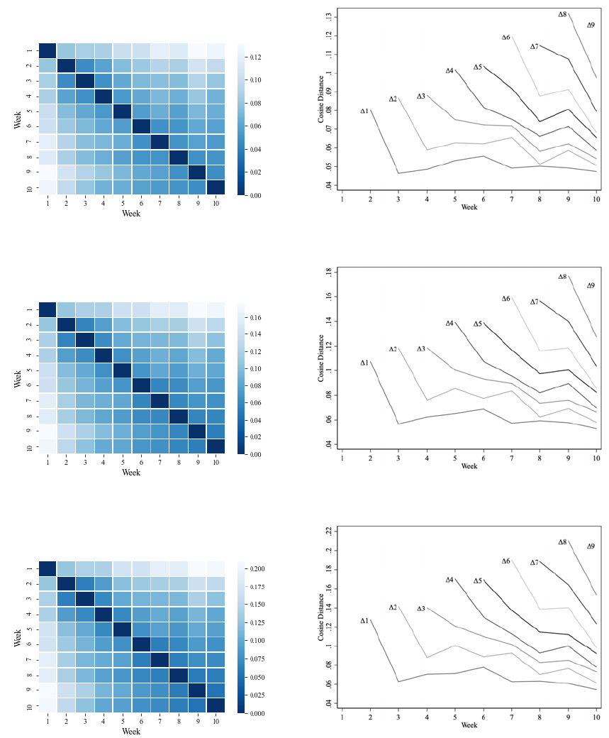
Figure A-4: Heat Maps and Oﬀ-Diagonal Figures for Repeat Sellers

(a) 2+ Messages (b) 2+ Messages

(e) 4+ Messages (f) 4+ Messages

Notes: This ﬁgure depicts heat map results and plots along the oﬀ-diagonals of those heat maps representing the

cosine distance of message bigrams across the ten weeks following May 25, 2016 for diﬀerent subgroups of sellers.

Panels (a) and (b) shows the results for sellers that have sent two or more messages during our sample period, Panels

(b) and (c) shows the same results for sellers that sent more than 3 messages, Panel (d) and (e) display the results

for sellers that appear four or more times in our messaging dataset.

Appendix-19

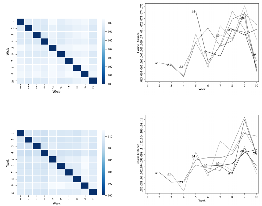
Figure A-5: Buyers and Sellers with No Experience

(a) Buyer Heat Map (b) Buyer Convergence

Notes: This ﬁgure depicts heat map results and plots along the oﬀ-diagonals of those heat maps representing the cosine

distance of message bigrams across the ten weeks following May 25, 2016 for buyers and sellers in our messaging dataset

that only sent one message. Panels (a) and (b) shows the results for buyers who sent one message within our sample

period and Panels (b) and (c) show the same results for sellers.

Appendix-20

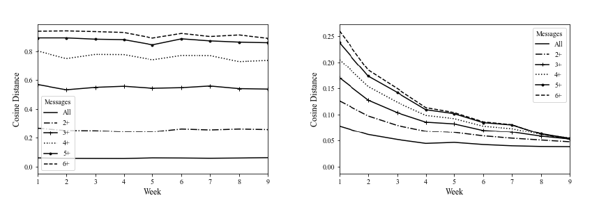
Figure A-6: The Bottom Gradient for Buyers and Sellers with Diﬀerent Experience

Levels

(a) Buyer (b) Seller

Notes: This ﬁgure presents the cosine distance between the messages sent in weeks x and 10 for buyers, Panel (a), and

sellers, Panel (b). Each panel is cut by groups, where All represents our results from buyer/seller messages for our

entire sample of buyers/sellers, 2+ from our sample of messages sent by buyers/sellers who sent 2 or more messages,

3+ from our sample of messages sent by buyers/sellers who sent 3 or more messages, and so on.

Appendix-21

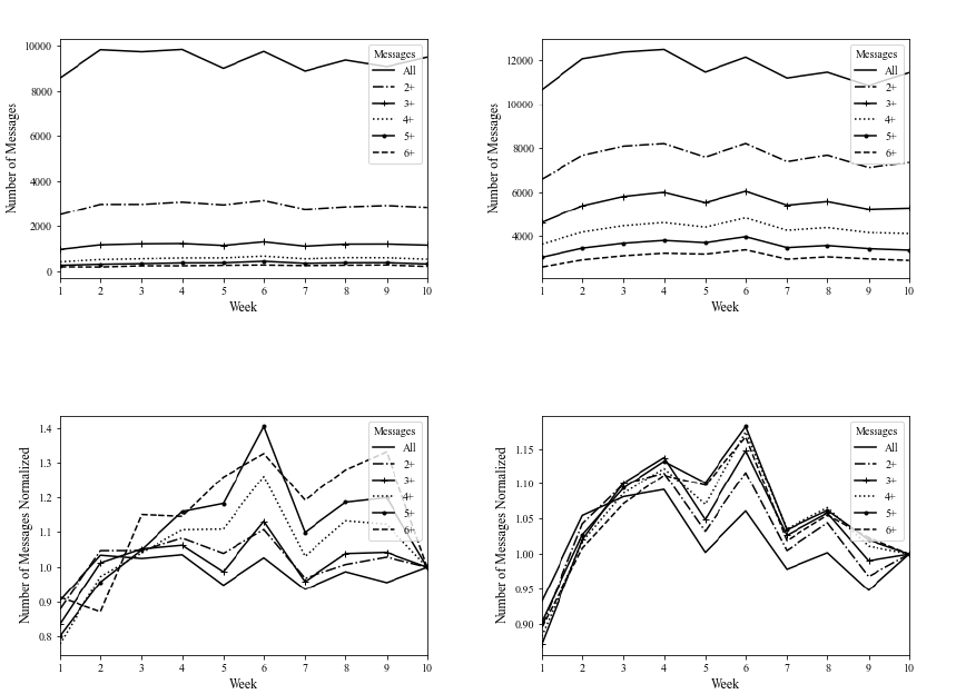
Figure A-7: Total Messages by Week for Buyers and Sellers

(a) Buyer (b) Seller

Notes: This ﬁgure presents the total number of messages sent by buyers, Panel (a), and sellers, Panel (b), by week.

Panel (c) and Panel (d) are the buyer and seller number of messages scaled by the number of messages in week 10.

Each panel is cut by groups, where All represents our results from buyer/seller messages for our entire sample of

buyers/sellers, 2+ from our sample of messages sent by buyers/sellers who sent 2 or more messages, 3+ from our

sample of messages sent by buyers/sellers who sent 3 or more messages, and so on.

Appendix-22

Table A-7: Top and Bottom Bigrams Correlated with Message Number

τ Nonzero Bigrams

Top 10

3 152

thanks in advance mfg; award-understand; understand beg; without eba; low

number of pieces; pray thanks; discount safeguarded; lg [NAME]; mfg sale; known

does

dank vorausmfg; preis versteh; versteh bitt; ohn eba; gering stuckzahl; bitt dank; rabatt

gewahrt; lg [NAME]; mfg verkauf; kund tut

1 1730

so far; thanks in advance mfg; beg functional scope of supply; observe scope

of delivery; Regular price insof; lg [NAME]; down selling price; shipping cost

adjusted; award-understand; low number of pieces

insof schon; dank vorausmfg; bitt funktionslieferumfang; funktionslieferumfang beacht;

verkaufspreis insof; lg [NAME]; runt verkaufspreis; versandkost angepasst; preis versteh; ger-

ing stuckzahl

0.5 3603

beg functional scope of supply; observe scope of delivery; Regular price insof;

thanks in advance mfg; so far; down selling price; lg [NAME]; award-understand;

shipping cost adjusted; discount safeguarded

bitt funktionslieferumfang; funktionslieferumfang beacht; verkaufspreis insof; dank vo-

rausmfg; insof schon; runt verkaufspreis; lg [NAME]; preis versteh; versandkost angepasst;

rabatt gewahrt

0.1 6290

Regular price insof; beg functional scope of supply; so far; observe scope of

delivery; lg [NAME]; shipping cost adjusted; down selling price; rather tight;

Newly listed; sale mfgruss

verkaufspreis insof; bitt funktionslieferumfang; insof schon; funktionslieferumfang beacht; lg

[NAME]; versandkost angepasst; runt verkaufspreis; recht knapp; neu eingestellt; verkauf

mfgruss

Bottom 10

3 152

counter already; gb memory card; miss it not; from august; for ﬁgure; sale

however; greeting [NAME]; over-looking payment method; ready priced; far kart

entgeg schon; gb speicherkart; verpass nicht; ab august; fur ﬁgur; verkauf jedoch; gruss

[NAME]; uberweis zahlungsmethod; bereit preislich; weit kart

1 1730

counter already; is set; gb memory card; ready priced; greeting [NAME]; just

give; extremely fair; suggest price proposal; not worn; month old

entgeg schon; eingestellt wurd; gb speicherkart; bereit preislich; gruss [NAME]; geb einfach;

ausserst fair; preisvorschlag ordnung; nicht getrag; monat alt

0.5 3603

woman has; is set; counter already; day would like; interess shipping; cm wide;

extremely fair; natural possible; ready priced; just give

freu schon; eingestellt wurd; entgeg schon; tag mocht; interess versand; cm breit; ausserst

fair; natur moglich; bereit preislich; geb einfach

0.1 6290

woman has; cm wide; day would like; under asking price; new mature; extremely

fair; dear interested person; is set; brand new unworn; rims tires

freu schon; cm breit; tag mocht; unt preisvorstell; neu reif; ausserst fair; lieb interessentin;

eingestellt wurd; nagelneu ungetrag; felg reif

Notes: This table includes the top and bottom ten bigrams in both English and the original German ranked by our

coeﬃcients on message number for diﬀerent levels of τ . The second column in the table indicates the amount of

message number coeﬃcients that are not penalized to zero for that value of τ .

Appendix-23

Table A-8: Top Messages

τ Nonzero Top Messages

152 1. this is our lowest price, please understand, many thanks in advance ... mfg (60)

dies ist unser niedrigster preis, verstehen sie bitte, vielen dank im voraus...mfg

2. hello, this product we played 20 % discount, and the price is already miss you please understand,

many thanks in advance ... mfg (20)

hallo, dieses produkt haben wir 20% rabatt gespielt, und der preis ist bereits mit verlust verstehen sie bitte, vielen

dank im voraus...mfg

3. they have slight problems when assessing the price but I understand that! (380)

sie haben leichte probleme beim einsch¨atzen des preises aber ich verstehe das!

1 1730

1. thank you for your price suggestion, but unfortunately it is below my purchase price: 10% ebay

commission, shipping, etc. are still going down and the selling price is calculated quite tightly.

please also note the scope of functions / scope of delivery! kind regards (40)

danke f¨ur ihren preisvorschlag, liegt aber leider unter meinem einkaufspreis: 10% ebay-provision, versand usw.

gehen ja auch noch runter und der verkaufspreis ist insofern schon recht knapp kalkuliert. bitte auch funktions-

/lieferumfang beachten! mfg

2. this is our lowest price, please understand, many thanks in advance ... mfg (60)

dies ist unser niedrigster preis, verstehen sie bitte, vielen dank im voraus...mfg

3. hello, this product we played 20 % discount, and the price is already miss you please understand,

many thanks in advance ... mfg (20)

hallo, dieses produkt haben wir 20% rabatt gespielt, und der preis ist bereits mit verlust verstehen sie bitte, vielen

dank im voraus...mfg

0.5 3603

1. thank you for your price suggestion, but unfortunately it is below my purchase price: 10% ebay

commission, shipping, etc. are still going down and the selling price is calculated quite tightly.

please also note the scope of functions / scope of delivery! kind regards (40)

danke f¨ur ihren preisvorschlag, liegt aber leider unter meinem einkaufspreis: 10% ebay-provision, versand usw.

gehen ja auch noch runter und der verkaufspreis ist insofern schon recht knapp kalkuliert. bitte auch funktions-

/lieferumfang beachten! mfg

2. this is our lowest price, please understand, many thanks in advance ... mfg (60)

dies ist unser niedrigster preis, verstehen sie bitte, vielen dank im voraus...mfg

3. hello, this product we played 20 % discount, and the price is already miss you please understand,

many thanks in advance ... mfg (20)

hallo, dieses produkt haben wir 20% rabatt gespielt, und der preis ist bereits mit verlust verstehen sie bitte, vielen

dank im voraus...mfg

0.1 6290

1. thank you for your price suggestion, but unfortunately it is below my purchase price: 10% ebay

commission, shipping, etc. are still going down and the selling price is calculated quite tightly.

please also note the scope of functions / scope of delivery! kind regards (40)

danke f¨ur ihren preisvorschlag, liegt aber leider unter meinem einkaufspreis: 10% ebay-provision, versand usw.

gehen ja auch noch runter und der verkaufspreis ist insofern schon recht knapp kalkuliert. bitte auch funktions-

/lieferumfang beachten! mfg

2. to get big discount, please send inquiry to delivery address directly to our e-mail. thank you

and friendly greetings, [NAME] [NAME] [company] [address] celle phone: xxxxx xxxxxxx email:

[email protected] (100)

um großer rabatt zu bekommen, bitte senden sie anfrage mit lieferadresse direkt auf unsere e-mail. danke und

freundliche gr¨uße, [NAME] [NAME] [company] [address] celle telefon: xxxxx-xxxxxxx email: [email protected]

3. hello, thank you very much for your interest! I can oﬀer you the lock for 80+ postage if we do

not go to the auction. I pass the sales commission on to you. just send me a message! best regards

(90)

hallo, vielen dank f¨ur ihr interesse! ich kann ihnen das schloß f¨ur 80 + porto anbieten, wenn wir auf die auktion

verzichten. die gesparte verkaufsprovision gebe ich so an sie weiter. senden sie mir hierzu einfach eine nachricht!

beste gr¨uße

Notes: This table presents the top three messages based on the summation of the coeﬃcients on message number for

each bigram in the message for diﬀerent levels of τ . The second column in the table indicates the amount of message

number coeﬃcients that are not penalized to zero. We include the listing price in euros rounded to the nearest tens

place in parenthesis next to each message. Finally, the German version of the message is included below each English

translation.

Appendix-24

Table A-9: Bottom Messages

τ Nonzero Bottom Messages

3 152

1. good morning, thank you for your best oﬀer. like I get to meet them on my original award, 50 I

can still give so. so we would be able to meet in the middle us virtually. with the request for your

understanding! m (400)

guten morgen, herzlichen dank f¨ur ihren preisvorschlag. gerne komme ich ihnen auf meinen urspr¨unglichen preis

entgegen, 50 kann ich schon noch nachgeben. so w¨urden wir uns quasi in der mitte treﬀen k¨onnen. mit der bitte

um verst¨andnis! m

2. I just discovered a very small hole on the back, so the price is a little bit more accommodating

.... best regards! (20)

auf der r¨uckseite habe ich gerade ein ganz kleines l¨ochlein entdeckt, daher komme ich im preis etwas entgegen ... .

sch¨onen gruß!

3. good day, many thanks for your interest in the wardrobe stand of classicon. it is a very beautiful

piece of furniture in excellent condition. like I get to meet them in the award. beautiful greetings to

jump! (1350)

guten tag, vielen dank f¨ur ihr interesse an dem garderobenst¨ander von classicon. es handelt sich um ein sehr sch¨onen

m¨obelst¨uck in hervorragendem zustand. gerne komme ich ihnen im preis entgegen. sch¨one gr¨uße nach springe!

1 1730

1. love potential customer, I like to go even at 55 down, but since that is not further jacket made

of real leather and as well as not being worn. I ask for understanding and would be happy about

their purchase still very! nice greetings, [NAME] [NAME] (60)

liebe interessentin, ich gehe gerne noch auf 55 runter, weiter jedoch nicht, da die jacke aus echtleder und so gut wie

nicht getragen ist. ich bitte um verst¨andnis und w¨urde mich ¨uber ihren kauf trotzdem sehr freuen! sch¨one gr¨uße,

[NAME] [NAME]

2. Suggest Price is ok, but please note notebook holidays. Shipping only possible again from 19:08.

if that’s okay, please buy. (10)

preisvorschlag ist in ordnung, bitte aber urlaubsnotiz beachten. versand erst wieder ab dem 19.08 m¨oglich. wenn

das okay ist, bitte kaufen.

3. since the book was purchased completely new and is not available in the book trade, I ask for

understanding that I no longer priced under these above-mentioned Suggest Price can go. I hope

they can also make friends with my proposal against. (10)

da das buch v¨ollig neu gekauft wurde und im buchhandel nicht erh¨altlich ist, bitte ich um verst¨andnis, das ich preislich

nicht mehr unter diesen o.g. preisvorschlag gehen kann. ich hoﬀe, sie k¨onnen sich mit meinem gegenvorschlag auch

anfreunden.

0.5 3603

1. love potential customer, I like to go even at 55 down, but since that is not further jacket made

of real leather and as well as not being worn. I ask for understanding and would be happy about

their purchase still very! nice greetings, [NAME] [NAME] (60)

liebe interessentin, ich gehe gerne noch auf 55 runter, weiter jedoch nicht, da die jacke aus echtleder und so gut wie

nicht getragen ist. ich bitte um verst¨andnis und w¨urde mich ¨uber ihren kauf trotzdem sehr freuen! sch¨one gr¨uße,

[NAME] [NAME]

2. I myself had EUR 80.00 plus shipping paid now for it: shipping included insured EUR 70.00. I

would be happy if the beautiful part is in good hands! kind regards! (80)

ich selbst hatte euro 80,00 plus versand bezahlt, f¨ur sie nun: euro 70,00 inklusive versicherter versand. ich w¨urde

mich freuen, wenn das sch¨one teil in gute h¨ande kommt! herzliche gr¨uße!

3. since the book was purchased completely new and is not available in the book trade, I ask for

understanding that I no longer priced under these above-mentioned Suggest Price can go. I hope

they can also make friends with my proposal against. (10)

da das buch v¨ollig neu gekauft wurde und im buchhandel nicht erh¨altlich ist, bitte ich um verst¨andnis, das ich preislich

nicht mehr unter diesen o.g. preisvorschlag gehen kann. ich hoﬀe, sie k¨onnen sich mit meinem gegenvorschlag auch

anfreunden.

0.1 6290

1. love potential customer, I like to go even at 55 down, but since that is not further jacket made

of real leather and as well as not being worn. I ask for understanding and would be happy about

their purchase still very! nice greetings, [NAME] [NAME] (60)

liebe interessentin, ich gehe gerne noch auf 55 runter, weiter jedoch nicht, da die jacke aus echtleder und so gut wie

nicht getragen ist. ich bitte um verst¨andnis und w¨urde mich ¨uber ihren kauf trotzdem sehr freuen! sch¨one gr¨uße,

[NAME] [NAME]

2. I myself had EUR 80.00 plus shipping paid now for it: shipping included insured EUR 70.00. I

would be happy if the beautiful part is in good hands! kind regards! (80)

ich selbst hatte euro 80,00 plus versand bezahlt, f¨ur sie nun: euro 70,00 inklusive versicherter versand. ich w¨urde

mich freuen, wenn das sch¨one teil in gute h¨ande kommt! herzliche gr¨uße!

3. sorry, but there is my lowest painful limit because the shoes have well over EUR 150 cost. I

would be happy if the beautiful shoes treat anyway. me they are unfortunately too small. (60)

sorry, aber da ist meine unterste schmerzgrenze, da die schuhe weit ¨uber eur 150 gekostet haben. w¨urde mich freuen,

wenn sie sich die sch¨onen schuhe trotzdem g¨onnen. mir sind sie leider zu klein.

Notes: This table presents the bottom three messages based on the summation of the coeﬃcients on message number

for each bigram in the message for diﬀerent levels of τ . The second column in the table indicates the amount of

message number coeﬃcients that are not penalized to zero. We include the listing price in euros rounded to the

nearest tens place in parenthesis next to each message. Finally, the German version of the message is included below

each English translation.

Appendix-25

Table A-10: Message Success (All Sellers)

(1) (2) (3)

Sim(m, week 10) 0.0456

∗

0.0345

∗

-0.0277

(0.0168) (0.0170) (0.0352)

Message Length 0.0009

∗

0.0002

(0.0002) (0.0004)

N 113600 113600 73839

Controls X X X

Seller FE X

Notes: This table presents our results from regressing message success onto a measure of seller experience. Sim(m,

week 10) is the cosine similarity between a message and the set of week 10 messages. All models include our main set

of controls: time trend; ln(ask price); category by condition ﬁxed eﬀects; day of week, precipitation, holiday dummies,

and the temperature. Model (3) includes seller ﬁxed eﬀects. Robust standard errors are reported in parentheses and

∗

denotes statistical signiﬁcance at α = 0.05.

Table A-11: Message Success (Sellers with Fewer than 11 Messages)

(1) (2) (3)

Sim(m, week 10) 0.0589

∗

0.0485

∗

0.0671

(0.0235) (0.0236) (0.0457)

Message Length 0.0014

∗

0.0003

(0.0002) (0.0005)

N 95617 95617 55903

Controls X X X

Seller FE X

Notes: This table presents our results from regressing message success onto a measure of seller experience. Sim(m,

week 10) is the cosine similarity between a message and the set of week 10 messages excluding sellers who sent more

than 11 messages. All models include our main set of controls: time trend; ln(ask price); category by condition ﬁxed

eﬀects; day of week, precipitation, holiday dummies, and the temperature. Likewise, all models drop sellers sending

more than 10 messages. Model (3) includes seller ﬁxed eﬀects. Robust standard errors are reported in parentheses

and

∗

denotes statistical signiﬁcance at α = 0.05.

Appendix-26